
Two rows of a random matrix can match by accident. When they do, the matrix loses its inverse. But rows can also depend on one another in less obvious ways, and symmetry ties their entries together. Can all those other dependencies make singularity exponentially more likely than one matching pair? OpenAI’s October 3, 2026 preprint answers for symmetric matrices built from fair signs. At dimension , the probability of singularity is . The exponent is up to a correction smaller than linear in . The proof gets there by asking which columns can break an invertible block, then measuring the arithmetic that makes such columns possible.
Table of Contents
1. What Is a Random Matrix and When Does It Become Singular?
A random matrix is a matrix drawn from a probability distribution. A singular matrix is a square matrix with no inverse. Over the reals, this is equivalent to having determinant zero and to having linearly dependent rows. Its corank is the dimension minus the rank, or the dimension of its kernel.
| Question | Result |
|---|---|
| Matrix model | Symmetric matrix with independent fair signs on and above the diagonal |
| Failure event | Zero determinant over the reals |
| Sharp rate | at dimension |
| Lower-bound event | Two specified rows are identical |
| Manuscript | OpenAI preprint, October 3, 2026 |
Take a two-by-two matrix with all four entries equal to 1. Both rows measure the same sum, so the vector is sent to zero. Change just the bottom-right entry to −1 and the two rows now measure the sum and the difference. The determinant is −2, so either input can be recovered from the two outputs. In higher dimensions even distinct rows can be dependent. The determinant detects those failures as well.
2. The Symmetric Bernoulli Matrix Problem
Write for an symmetric Bernoulli matrix. Draw an independent fair sign for every position on or above the diagonal, then copy each off-diagonal entry into its mirror position. This random symmetric matrix uses independent signs. The entry in position supplies both row and row , so two different rows share a random variable even though every entry within a given row is marginally a fair sign.
Discreteness makes the question matter. If the upper-triangular entries instead have a joint density, the zero set of the determinant polynomial has probability zero. The polynomial is nonzero because it takes value 1 at the identity. The sign model puts positive probability on individual matrices, including singular ones. Exact rank loss can therefore survive at every dimension.
3. OpenAI’s Sharp Exponential Singularity Theorem
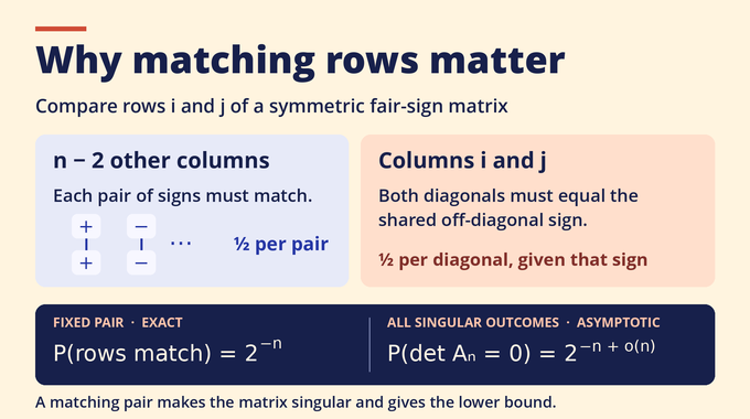
Theorem 1.1 in the October 3 manuscript gives the following rate, where denotes the singularity probability.
Here tends to zero. In the exponent, denotes a term whose ratio to tends to zero. Thus the base-two log probability divided by the dimension tends to −1, even if factors that vanish or grow subexponentially multiply .
For two fixed rows, the entries outside their two column positions must match pairwise. At the two remaining positions, both diagonal signs must equal the shared off-diagonal sign. Conditional on that shared sign, each diagonal condition costs a further factor of one half. This gives the exact probability for and supplies the lower bound.
4. Why the Symmetric Case Resisted Earlier Methods
The corresponding result in random matrix theory concerns a sign ensemble with every entry independent. There, exposing one row leaves the distribution of the next row intact. Konstantin Tikhomirov obtained the sharp rate for that ensemble. In the symmetric case, a revealed row also reveals part of every future row. When the last row and column are appended together, the fresh signs enter a quadratic form rather than a single linear sum.
Littlewood–Offord theory asks how much probability a random sum can put on a particular value. Costello, Tao, and Vu developed quadratic versions of that idea and showed that the symmetric singularity probability tends to zero. Later work improved the decay, and Campos, Jenssen, Michelen, and Sahasrabudhe bounded it by for some fixed . That gave exponential decay. OpenAI’s theorem identifies its leading constant in the exponent, namely the natural logarithm of 2.
5. The Complete Proof Strategy: From Coin Flips to Arithmetic Structure
OpenAI’s release announcement attributes the collection to an internal frontier model and discusses Lean formalizations across the release. The manuscript’s repository entry records its authorship and citation. The six stages below reconstruct the written proof from the manuscript, which presents the logical argument without a discovery chronology.
- Reduce the model. Use the first row and column to exchange signs for bits while preserving the chance of singularity.
- Isolate the last column. Reduce to one missing rank and delete a coordinate to get an invertible block. Count the new columns that make the enlarged matrix singular.
- Organize candidates arithmetically. Group columns by the fractions introduced by the inverse. Summarize the repeated prime-power structure in a potential.
- Bound the count for a fixed block. Use the geometry of candidate columns to show how much arithmetic structure a large count would require.
- Price the structure as the block grows. Show that retaining many arithmetic constraints uses up probability when new bits are drawn.
- Average along paths of minors. Combine the extension costs along paths. This bounds the expected column count and gives the sharp probability bound.
6. Schur Complements and the Reduction to Admissible Columns
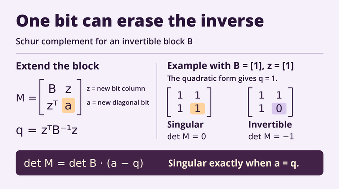
First, scale the sign matrix by its first diagonal sign, then flip matching rows and columns to make the first row and column all ones. Conditional on the original first row, the lower block still consists of independent fair signs on and above its diagonal. Eliminating the first coordinate subtracts 1 from every entry of that block. The remaining entries are 0 or −2, giving with . The two models have equal singularity probabilities at these paired dimensions.
A rank estimate makes corank above negligible. For positive corank at most that threshold, flipping suitable diagonal bits leaves exactly one kernel direction. The flipped locations recover the original matrix and have only subexponentially many possible choices. Now remove an index where a corank-one kernel vector has largest absolute coordinate. The remaining principal block is invertible. The kernel equations force the new diagonal bit and bound the largest absolute entry of by 1.
Here is the extended matrix, its new bit column outside the diagonal, and the superscript denotes transpose. For a concrete example, take and . Then , so the new diagonal bit makes the extended matrix all ones. With the determinant becomes −1. In general, contains precisely the bit columns for which the quadratic form is a bit and the inverse-image bound holds. Each such column fixes one diagonal bit. Summing over the candidate deleted indices gives the bound in Lemma 2.5.
7. Discriminant Groups and the Arithmetic Potential
The inverse can introduce fractions. Adding a vector from to changes by an integer vector, so the possible fractional parts live in the discriminant group . It has elements. The pairing sends classes to . It is well defined because changing either representative changes the value by an integer. An admissible column pairs to zero with itself, since its quadratic form is a bit. Pairings between different columns can still be nonzero.
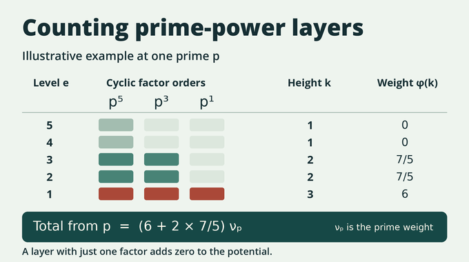
Decompose the group into cyclic prime-power factors. For prime and level , the layer height counts factors at that prime with order at least . Imagine one stack per factor. The height at level counts how many stacks reach it. The potential charges no weight for heights zero and one, uses for height two, and uses for height . With prime weight , the paper defines
For prime exponents 5, 3, and 1, the heights are 3, 2, 2, 1, and 1. Their contribution is . Hadamard’s determinant bound gives in the dimensions used by the proof.
8. Lattice Geometry and the Static Admissible-Column Bound
Zero self-pairing alone can leave a large collection of columns. The paper splits those classes into groups whose differences have controlled pairings. From a largest group it extracts a robust subset. Roughly, its points are spread across their affine span, so restricting to lower-dimensional slices cannot preserve too large a share. The differences of the graph points generate a lattice. The inverse-image bound keeps them short, and robustness bounds the lattice’s covolume, the volume of a fundamental cell in its span.
The pairing gives a lower bound for the absolute determinant of a nondegenerate part of the restricted form. The graph metric changes each eigenvalue of the inverse form from to . This prevents tiny eigenvalues of from creating large eigenvalues of the graph form. A spectral estimate gives an upper determinant bound. A finite cover of rational subspaces of controlled height makes the needed rank bound hold even though the span was selected after seeing the matrix. Comparing the determinants limits its dimension, and an affine span of dimension contains at most cube vertices.
The Reverse Minkowski theorem of Regev and Stephens-Davidowitz supplies a short-vector estimate in the proof’s lattice toolkit. The paper applies it to the orthogonal quotient after removing a determinant-minimizing sublattice at the chosen scale. Accounting for the grouping cost and span dimension gives Proposition 2.6. Write and let be any fixed positive precision exponent. For typical nonsingular matrices of sizes between and ,
9. Certificate Pricing and the Cost of Arithmetic Structure
A large potential can allow many admissible columns. To control how often that happens, the paper tracks what survives when a nonsingular block grows by one coordinate to a nonsingular block . The two discriminant groups share a quotient. On the starting side it is obtained by factoring out the class of the new column . Each layer height drops by at most one in that quotient. Within a run of equal original heights, the layers that keep their height form an initial segment. Symmetric extension identities and kernel counts modulo prime powers help control the layers of the destination group.
Demanding retention of selected layers forces into a particular integer lattice. Large lattice index alone does not guarantee few points in the bit cube. The paper proves a simultaneous bound on those intersections for lattices containing . A partial certificate names a subset of retained layers. Naming more layers imposes stronger constraints, while giving more possible certificates to count. Optimizing the certificate size balances those effects. At width one, the probability cost offsets the potential increase in the conditional expectation of .
10. Principal-Minor Paths and the Final Probability Bound
An invertible principal minor can be found by deleting one index when the inverse has a nonzero diagonal entry. If all its diagonal entries vanish, deleting two indices at a largest-magnitude off-diagonal entry of the inverse works. In the two-index case, both cross columns must be admissible when the step is read forwards. Conditional on the old block they are independent, so the chance of passing this gate is the square of the admissible fraction. The static estimate supplies the needed probability cost.
The proof constructs paths backwards to cover the outcomes, then estimates each fixed path forwards so newly revealed bits remain independent. A long initial segment makes a large tail of high layers unlikely near the end. Tracing a tail backwards raises the height threshold at each step until a uniform bound on corank modulo every prime rules it out. A large tail near the end would therefore require substantial retention along that segment.
In the short terminal window, reaching small potential lets the conditional estimate control the rest. If potential stays large despite a small high-layer tail, a bounded statistic must decrease at each cheap step. It cannot keep decreasing across the window, so the path must make many steps that retain substantial weight or pass an expensive two-column gate. Their conditional probabilities make this alternative negligible.
The path count costs only a subexponential factor. Proposition 2.7 bounds the expected weight, using an indicator that is one on nonsingular outcomes and zero otherwise.
Combined with Proposition 2.6 and the negligible exceptional set, this yields . The corank reduction then gives as an upper bound for the binary singularity probability. A specified zero row gives the matching lower exponential rate, and the sign-to-bit equality returns Theorem 1.1.
11. Testing Random Matrix Singularity With a Computational Experiment
The table below is an independent illustration. For dimensions 2 through 5, enumerate every upper-triangular sign pattern in row order, including the diagonal, and mirror the signs. For dimensions 8, 12, and 16, draw 4,096 matrices at each size. To reproduce the sample, initialize Python’s random.Random(20261003) once, visit those sizes in order, and take each sign as twice getrandbits(1) minus one.
| Dimension | Method | Singular / Total | Share |
|---|---|---|---|
| 2 | Exact | 4 / 8 | 50% |
| 3 | Exact | 32 / 64 | 50% |
| 4 | Exact | 512 / 1,024 | 50% |
| 5 | Exact | 15,872 / 32,768 | 48.44% |
| 8 | Sample | 1,309 / 4,096 | 31.96% |
| 12 | Sample | 534 / 4,096 | 13.04% |
| 16 | Sample | 93 / 4,096 | 2.27% |
Classify rank by Gaussian elimination over the prime field of order . For the tested dimensions, Hadamard’s inequality gives , so zero determinant modulo this prime is equivalent to zero over the integers. This avoids confusing a small floating-point pivot with exact rank loss. The frequencies decline in the sampled range, while the exact small-size results show how far finite-dimensional probabilities can sit above the contribution from a single matching pair.
12. What OpenAI’s Proof Establishes and What Remains Open
For this fair-sign ensemble, the random matrix singularity theorem fixes the exponential rate. A sharper asymptotic would quantify the multiplier in front of and determine how much of the probability comes from elementary row dependencies. Numerical conditioning is a separate question. A nonsingular matrix can still have a very small positive least singular value, which can amplify rounding errors or perturbations when solving a linear system.
The proof’s main insight is that a column capable of producing exact rank loss faces two constraints at once. Its quadratic form must match the diagonal bit, and its inverse image must stay in a bounded cube. Together those constraints let lattice geometry and arithmetic turn a global rank question into a count that can be averaged. Follow Binary Verse AI for more research explainers, from random 3-SAT thresholds and critical percolation to Ramanujan graph spectra and exact Fourier transform complexity.
What is a random matrix?
A random matrix is a matrix whose entries are generated according to a probability distribution. In OpenAI’s research, entries on and above the main diagonal independently take values of −1 or +1 with equal probability, while the remaining entries are determined by symmetry.
What is a singular matrix?
A singular matrix is a square matrix that has no inverse. Its determinant is zero, its rows and columns are linearly dependent, and its rank is smaller than its dimension.
What is a Bernoulli matrix?
A Bernoulli matrix is a random matrix constructed using entries with two possible values, commonly 0 and 1 or −1 and +1. OpenAI’s manuscript studies symmetric matrices with uniform random signs and reduces them to a corresponding binary model.
What did OpenAI prove about random matrix singularity?
For an n-by-n symmetric matrix with independent fair signs on and above the diagonal, OpenAI proved that the singularity probability equals one half plus a term tending to zero, with that sum raised to the nth power. This gives the sharp exponential decay rate as the dimension grows.
Why are symmetric random matrices harder to analyze?
Symmetry creates dependencies between rows and columns because every off-diagonal entry appears twice. Consequently, probability arguments that rely on independent rows cannot be directly applied.
Is OpenAI’s singularity probability an exact formula?
No. The theorem fixes the leading exponent in base two at minus the dimension, up to a correction smaller than linear in the dimension. The exact probability at each size and the precise multiplier of 2 to the power of minus the dimension remain undetermined by this theorem.
Are nonsingular random matrices always numerically stable?
No. A nonsingular matrix can have a very small positive least singular value, which can amplify errors in numerical inversion or when solving a linear system. The theorem concerns exact singularity.