
Imagine two routes across a honeycomb grid, each exactly a thousand steps long and each forbidden to touch a vertex twice. One can curl back toward its start while the other reaches across the grid. How much space does a typical route occupy? OpenAI’s manuscript proves that a uniformly sampled -step self-avoiding walk on the honeycomb lattice has Euclidean diameter . Its local vertex counts and covering numbers obey the corresponding scaling law simultaneously across locations and scales. The proof links a decades-old prediction about polymers to estimates on paths that cross strips, then carries those estimates back to walks of each sufficiently large integer length.
Table of Contents
1. What Is a Self-Avoiding Walk?
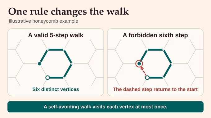
The honeycomb lattice consists of the vertices and edges of a regular hexagonal tiling. Each vertex has three neighbors. Connecting the centers of neighboring triangles in the triangular tiling gives the same lattice. A self-avoiding walk takes nearest-neighbor steps and keeps every visited vertex distinct. For example, it can follow five consecutive edges around one hexagon, but following the sixth would return it to its starting vertex. An ordinary random walk can make that return or even reverse its first step immediately.
| Quantity | Meaning | Proven Scale |
|---|---|---|
| Diameter | Greatest Euclidean distance between any two visited vertices | up to power slack |
| Local mass | Number of visited vertices within radius of a visited vertex | up to power slack |
| Covering number | Fewest closed balls of radius that cover the vertices, with centers anywhere | up to power slack |
The paper fixes the starting vertex and samples uniformly from all valid paths of length , with a free endpoint. A kinetic walk instead chooses from the unused neighbors at each step. It can run out of choices, and even among paths that survive to length , the products of the step probabilities can differ. This distinction matters when interpreting a simulation of a self-avoiding random walk.
2. The Decades-Old Mystery of the 3/4 Exponent
A lattice walk models a polymer in a simplified setting. Consecutive monomers occupy neighboring sites, and excluded volume prevents two monomers from sharing a site. The predicted two-dimensional self-avoiding walk exponent comes from Bernard Nienhuis’s 1982 analysis of the dilute loop model in the limit of zero loop weight. At the level of exponents, quadrupling the chain length multiplies its spatial extent by . The diffusive scale of an ordinary planar random walk grows by a factor of two under the same change.
Duminil-Copin and Smirnov determined the exact honeycomb connective constant, the exponential growth rate of the number of walks. That answers a counting question. Knowing the growth rate alone leaves open which shapes account for most of the count. Later work by Krachun and Panagiotis gave a quantitative sub-ballistic bound, showing that the walk stays within order of its origin with high probability. This still allows spatial scales much larger than the predicted .
3. What OpenAI’s Self-Avoiding Walk Proof Establishes
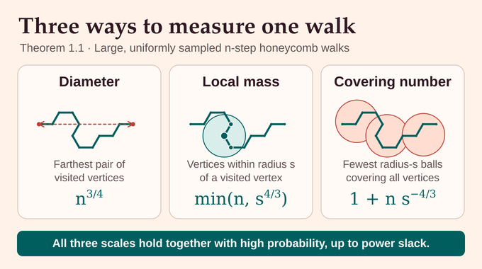
In Theorem 1.1, denotes the path, counts its edges, is a visited vertex, and is a Euclidean radius. For any exponent slack and any failure exponent , there is a constant such that, for every sufficiently large integer , all three bounds hold on one event of probability at least .
The mass and cover bounds hold for every real and, for mass, every visited . The in the diameter exponent represents an error smaller than any fixed in this probability sense. The bounds specify powers and allow slowly varying multiplicative factors. The theorem also leads to a lower bound of on the walk’s projected span along each of the three lattice normals.
4. The Complete Proof Strategy From Critical Weights to Fixed-Length Walks
The following six stages reconstruct the published proof. OpenAI’s release announcement attributes the results to an internal frontier model. Its repository describes the broader evaluation process and lists the families with public reasoning summaries. Family 237, the honeycomb walk family, is absent from that list. The stages below follow the dependencies visible in the manuscript.
- Make cuts affordable. Give longer paths smaller weights and bound the sum of all path weights in a box. When a troublesome segment is cut out, the pieces on either side can then be summed at a controlled cost.
- Build long bridges that fit. Use loops around a face to find long chords and glue those chords into bridges. Recover the joining lines to control how often any output has been counted.
- Repeat at fresh starts. A sufficiently long confined bridge may be rare. Restart at successive bridge cuts and use repeated trials to make a long segment likely before conditioning on a prescribed final height.
- Test consecutive pieces together. At each turn, the incoming and outgoing pieces must fit without crossing. Combining this constraint across turns suppresses both unusually fast and unusually slow travel.
- Count returns. A walk can leave a region and revisit it repeatedly. Convert many separate visits into disjoint crossings and bound their combined weight with a polygon count.
- Fix the length. Restrict the weighted estimate to edges and divide by the total weight at that length. Use the resulting subpath and local count bounds to control diameter and covering.
5. Parafermionic Observables and the Critical Geometry of Honeycomb Walks
The companion papers supply positive weighted estimates that the main manuscript uses as inputs. Write for the critical activity, the reciprocal of the connective constant. A vertex-rooted walk with edges has weight .
A strip bridge instead runs between ports, the midpoints where honeycomb edges cross the boundary lines. Its length counts visited vertices, including neither port. This lets adjacent pieces multiply their weights exactly. The parafermionic observable attaches a complex phase to a path’s signed turning. Local cancellation becomes a boundary flux identity on summation. In a strip, it relates the total weight of arches returning to the starting boundary to the weight of strict bridges crossing bands from one fixed port to any compatible terminal port. The quantitative input gives , where denotes comparison in both directions by fixed positive constants.
Three other inputs do different jobs. Nesting estimates count weighted disjoint loops around a face and supply bulk length through a comparison with chords through a marked edge. Marked polygon estimates control sums weighted by squared polygon length. A cylinder arc estimate bounds paths between two marked ports, even when the two groups of bands have very different sizes.
6. Controlling the Total Mass of Walks Inside a Box
After isolating a subpath, the proof has to pay for everything discarded. There can be exponentially many length-restricted paths, so counting the discarded pieces without regard to the weight gives little control. The full-box susceptibility instead sums critical weights for all lengths and endpoints in a box of side , from a fixed start, and then maximizes over starts. Proposition 3.1 bounds this quantity by a fixed polynomial in .
The reduction cuts out a middle arc whose earlier and later steps can serve as the two marks of a cylinder. The lattice directions near the marks put the arc within the companion estimate’s range. The prefix before the first useful mark is confined in parts to narrow strips. On long stretches away from those strips, its allowed steps have low enough growth that their critical weights sum to a bounded amount. A short terminal remainder costs only a constant. Paths that fail the suffix test contribute a small multiple of the very box mass being bounded. Absorbing that term leaves a polynomial bound. Later, arbitrary polynomial decay can absorb the price of restoring the outside pieces.
7. Building Confined Bridges Through Recoverable Cuts
A large mean length could result from a few extreme paths, and a strip of finite height still extends indefinitely sideways. The proof seeks long bridges whose diameters stay within a fixed multiple of their height. It attaches exterior connectors to chords carrying bulk length, then reads the seams back from the resulting bridge. Bounds on possible seam locations keep repeated representations from inflating the lower estimate.
For the second moment, the proof closes confined paths into polygons. For a bridge, the two recovery lines move together at fixed separation, limiting how many cuts can produce the same polygon. The resulting confined first-length mass is at least and the second at most . The first-length mass below , for any fixed , is too small to account for the first estimate. Weighted Cauchy–Schwarz gives the remaining long paths critical mass at least . Division by leaves a success probability of at least under the normalized bridge law.
8. Renewal Theory Turns Rare Long Bridges Into Reliable Estimates
A strict bridge reaches the opposite boundary with no other boundary visit. At a level it crosses exactly once, it can be cut into two strict bridges. Cutting at all such levels gives a unique sequence of irreducible bridges. The critical weights of individual irreducible pieces sum to one, so they can be sampled independently and joined in successive strips.
Each trial starts at a fresh cut and stops at the first renewal beyond a chosen height increment. The proof controls overshoots so many trials fit below the target height with high probability. It then conditions on an actual cut at height . Given a stopped prefix at height , the chance to hit the target is for , so the conditioning introduces an explicit weight ratio. The resulting bridge typically has length up to exponent slack, with polynomially small failure probability. A separate sewing construction provides turning corridors for the next stage, allowing a bridge to pass an obstacle while retaining usable critical mass.
9. Why Self-Avoiding Walks Cannot Spread Too Quickly or Too Slowly
Travel is fast when a path spans a large distance using too few edges. Cutting at successive turning extrema exposes bridge pieces. Near the joins, two arms must avoid each other. Ordered probes reveal the two renewal sequences and charge for continued avoidance. If tests from both ends inspect the same long irreducible piece, its critical weight enters once. Counting that piece as two independent samples would give an unjustified gain. To bound compatible arms, the argument sews qualified pairs into longer bridges with a recognizable U-turn. The output bridge mass and the number of ways to recover the turn constrain the weight of the original pairs.
The fast-travel argument combines avoidance at turns with the shortage of short bridges on large scales. The slow-travel argument deals with too many edges in a narrow span. Recursively cutting at extrema forces either a long chain of comparable pieces or many pieces that are themselves unusually long. Joint bounds for these configurations make each type of exception smaller than any prescribed inverse power of the box scale. The result controls every contiguous subwalk while leaving open how often the full walk can return to one ball.
10. Repeated Crossings and the Emergence of the 4/3 Mass Exponent
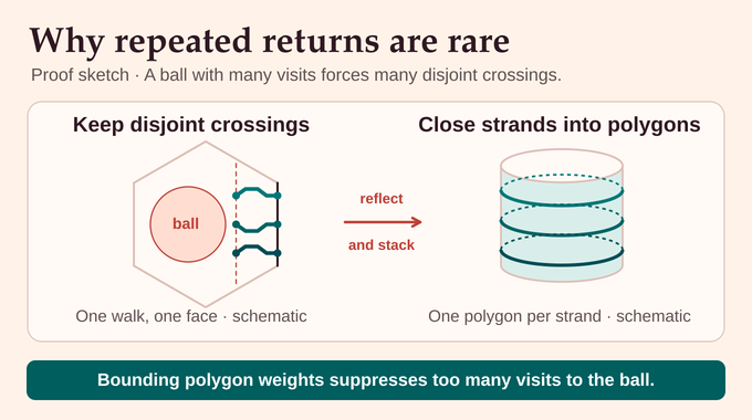
Surround the ball by a larger lattice hexagon. Group visits into batches that end when the path next hits the hexagon boundary, apart from a possible final batch at the walk’s endpoint. Each batch is confined to a region of diameter of order , so the subwalk bound limits its length. If the ball still has too many vertices, many batches must reach the same face. From each, retain the last crossing from an inner parallel line to that face.
These disjoint bridges can be reflected and stacked on a cylinder so that each strand closes into a separating polygon. The original strands are recovered by cutting at the prescribed levels. The logarithm of the polygon-count bound has a penalty of at least a constant times for crossings, sufficient to outweigh the order cost of choosing their endpoints and summing the complementary pieces once grows as a positive power of . This gives the local mass upper bound even when visits are widely separated in time.
11. The Final Transfer to Uniform Fixed-Length Walks
Let count the rooted -step walks. Their total critical weight is . Indeed, cutting a walk gives submultiplicativity. If the critical weight at any one length were below one, submultiplicativity would force exponential decay at large lengths, contradicting the polynomial strip-crossing mass. All -step walks fit in a box of scale proportional to . Dividing the exceptional critical mass at length by therefore preserves the arbitrary polynomial probability bound.
A short contiguous block through a visited vertex fits inside its radius- ball by the fast-travel bound, giving the local mass lower bound. Splitting the whole walk into such blocks gives a cover. Conversely, a covering ball that hits the trace fits inside a ball of twice the radius about a visited vertex, so it can cover only as many vertices as the local mass upper bound allows.
| At radius | Leading Power |
|---|---|
| Vertices per occupied ball centered on the walk | |
| Balls needed to cover the walk |
These are derived powers with theorem slack. The same covering law yields a logarithmic dimension of at scales separated from the walk’s diameter by a fixed power of its length. The radius of gyration , the root mean square distance from the visited vertices to their centroid, also has exponent . At a radius just below that scale, each vertex has only a vanishing fraction of the others nearby. The mean squared pairwise distance thus gives the lower bound, while the diameter gives the upper bound. Both size statistics have th moment exponent for every fixed .
12. What the Proof Resolves and What Remains Open
For two-dimensional polymer models, the proof gives a rigorous exponent for a fixed-length self-avoiding walk and shows how its vertices occupy space across scales. This discrete covering law gives precise meaning to the fractal dimension in the lattice setting. The conjectured continuum limit is , a random curve with Hausdorff dimension . The lattice result leaves continuum convergence, universality across lattices, and a matching lower bound on endpoint displacement open. A walk can have two far-apart vertices and still end close to its start.
OpenAI’s Lean scope note lists supporting results such as the strip-crossing mass and bridge summability. The fixed-length diameter, mass, and covering theorem is proved in the manuscript. For more research explainers, follow Binary Verse AI’s coverage of critical percolation, lattice spin models, and computer-checked results in percolation theory.
What is a self-avoiding walk?
A self-avoiding walk is a path along neighboring lattice vertices that never visits the same vertex twice. Unlike an ordinary random walk, its possible movements are constrained by its entire previous trajectory.
What did OpenAI prove about self-avoiding walks?
OpenAI proved that uniformly sampled, sufficiently long, fixed-length self-avoiding walks on the honeycomb lattice have diameter exponent 3/4 and simultaneous local-mass and covering exponents 4/3. The bounds allow arbitrarily small positive exponent slack and failure probability bounded by any prescribed inverse power of the walk length, up to a constant.
How far does a self-avoiding walk spread?
For the honeycomb lattice model studied in the paper, the diameter of an n-step walk scales as n to the power 3/4, up to arbitrarily small exponent slack with the theorem’s high-probability guarantee. This is faster than the typical square-root spatial scaling of an ordinary two-dimensional random walk.
Why is the mass dimension of a self-avoiding walk 4/3?
The exponent 4/3 is the reciprocal of the diameter exponent 3/4. The manuscript rigorously establishes this relationship through simultaneous bounds on local vertex counts and covering numbers. Those bounds describe the lattice trace. The existence of a continuum scaling limit and the Hausdorff dimension of such a limit are separate questions.
Can a self-avoiding walk become trapped?
A sequentially generated self-avoiding walk can become trapped when all neighboring vertices have already been visited. OpenAI’s manuscript studies a different probability model, the uniform distribution over all valid walks of a prescribed length.
Why are self-avoiding walks important in polymer physics?
Self-avoiding walks model polymer configurations in which different segments cannot occupy the same site. Their scaling exponents describe how the typical spatial size of a polymer changes with its chain length.
Does OpenAI’s proof apply to every two-dimensional lattice?
The proof applies to the honeycomb lattice and uses analytic estimates tied to its geometry. Universality across lattices, convergence to SLE with parameter 8/3, and the corresponding scaling law in three dimensions remain outside the theorem.