
A pair of molecules drawn into an attractive well can keep interacting long enough for a third to arrive. The Boltzmann equation still describes the dilute-gas limit of that Newtonian system under the conditions proved in OpenAI’s September 2026 manuscript. The result covers stable, finite-range radial forces in three dimensions, including potentials with attractive wells. It holds throughout any fixed finite interval on which the classical kinetic solution satisfies the required Gaussian velocity bound. The proof follows entire interacting groups, then shows why their extra correlations disappear from every fixed-order particle distribution in the limit.
Table of Contents
1. What Is the Boltzmann Equation?
The Boltzmann transport equation tracks a phase-space density , where is time, is position, and is velocity. Integrating over velocities gives the spatial density. Between encounters, particles stream through space with their current velocities. Encounters redistribute velocities according to the scattering law for the pair potential .
The left side measures the change in density along a freely moving trajectory. The operator on the right accounts for gains and losses caused by scattering. Its two density inputs reflect the incoming pair. The equation is nonlinear because the same evolving distribution supplies both.
| Particle Model | Three-dimensional Newtonian point particles with a random initial cloud and pair exclusion at time zero. |
|---|---|
| Forces | Stable radial potentials of finite range. Attractive wells and a repulsive singularity at the origin are allowed. |
| Time Window | Any fixed finite interval with a classical Boltzmann solution satisfying the theorem’s uniform Gaussian bound. |
| Result | Strong convergence of every fixed-order rescaled factorial marginal to the corresponding product density, uniformly in time. |
2. The Original Problem of Deriving Gas Dynamics From Newton’s Laws
Given the initial positions and velocities, Newton’s laws determine the trajectories. Kinetic theory starts with a distribution of initial configurations and asks what a typical cloud looks like after many encounters. A single-particle density can record where particles are and how fast they move. It cannot tell you which particles have already met or share a collision partner.
The molecular-chaos assumption closes the kinetic equation by using a product of one-particle densities to describe incoming pairs. But imagine two particles both hit by a third. The earlier collisions can connect their velocities even if those two particles have never met. Deriving the equation means justifying the product structure in the relevant limit despite these microscopic correlations. This is the kinetic step in a program associated with Hilbert’s sixth problem, which asks for rigorous links between descriptions at different scales.
3. Why Previous Boltzmann Equation Derivations Were Limited
Lanford’s theorem established the hard-sphere limit for short times. King treated positive finite-range potentials, and Pulvirenti, Saffirio, and Simonella later proved a short-time result for the stable radial class used here. The attractive part of a potential was already within reach. The challenge was controlling its effects across a full regular kinetic interval.
Deng, Hani, and Ma reached that interval for hard spheres by carrying correlation histories across time layers. Simply restarting a short-time proof would require control of the evolved input that the short-time result alone cannot supply. Smooth forces create another difficulty. An encounter occupies time, and several forces can act at once. A history of instantaneous binary collisions cannot record the potential energy of a group that stays together across a time cut.
4. What OpenAI’s New Boltzmann Equation Proof Establishes
Theorem A of the original manuscript starts from a normalized random cloud with initial pair exclusion. Its initial one-particle input is a nonnegative, continuously differentiable probability density. The density and its spatial gradient must have Gaussian velocity bounds whose local suprema are summable over space. The potential is fixed as the range shrinks. It is twice continuously differentiable, with an allowed repulsive singularity at the origin. The theorem assumes a nonnegative classical probability-density solution through time , with a uniform bound on for the same used in the initial bounds.
Here is the force range, and is any fixed positive integer. The density counts ordered selections of distinct particles, averages over the cloud, and rescales by , where is the activity. The tensor power is the product density for independent samples. The norm integrates the absolute difference over all their positions and velocities. The supremum requires one error bound across the observation interval. Corollary B applies this result to empirical averages of smooth, compactly supported tests.
5. The Complete Proof Strategy in Six Stages
OpenAI’s release announcement attributes the collection to an internal frontier model. The six stages below reconstruct the logic of the published manuscript. The mathematical argument for this result appears in the preprint.
5.1 Microscopic Foundations
Start with exact Newtonian trajectories and isolate a two-body encounter. The flux of particles entering the interaction sphere gives a scattering measure even when the outgoing angle is a complicated function of the initial approach.
5.2 Component Expansion
Cut time into fine cells and trace back the complete interacting groups needed to reconstruct the particles of interest. An exact signed expansion turns those dependencies into finite integrals over subsystem histories.
5.3 Layered Centering
At coarser time cuts, subtract the kinetic contribution from isolated single particles. Independent families cancel, so the residual histories retain the correlations the proof needs to estimate.
5.4 Common Energy Budget
Charge each formal particle lifetime for its source velocity once and use stability to bound the kinetic energy along the history. This lets the time integrals offset the cost of carrying velocities through repeated encounters.
5.5 Causal Exposure
Find fresh scattering parameters in disjoint parts of a history. Reveal them at the first extra contact, when the comparison trajectories are still determined independently of those parameters.
5.6 Kinetic Convergence
Use the geometric and energy estimates to control the finite expansion and the errors from stopping it. Then recover the full marginals from the separated configurations and conserved factorial mass.
6. The Boltzmann–Grad Limit and the Mathematics of Molecular Collisions
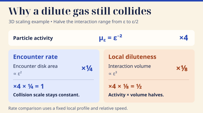
In three dimensions the activity is . For a scaling example, halve the range. The area of the encounter disk drops to one quarter, while the activity quadruples. At fixed local profile and relative speed, the two factors compensate. The volume within interaction distance shrinks by a factor of eight, so the activity times that volume halves. Encounters can occur at order-one frequency while the gas becomes dilute on the interaction scale.
The grand-canonical law assigns a cloud of size a product density weighted by , restricted to pair distances greater than , then normalizes across all sizes. The pair term in the Hamiltonian uses the rescaled potential .
Each and is the position and velocity of particle . Newton’s equations use the gradient of the original potential with respect to its argument. The factor comes from differentiating the rescaled potential.
At fixed range, the law gives a global finite-particle flow on its finite-energy domain. Stability means the total potential energy for particles is bounded below by with a fixed . This controls how much kinetic energy can come from attraction. Conservation of the Hamiltonian then bounds all speeds for a fixed cloud. In the singular case it also keeps any given pair away from zero separation. Pair exclusion applies at initialization. Later clusters evolve under the same forces as the rest of the cloud.
7. Deriving the Boltzmann Collision Integral From Particle Scattering
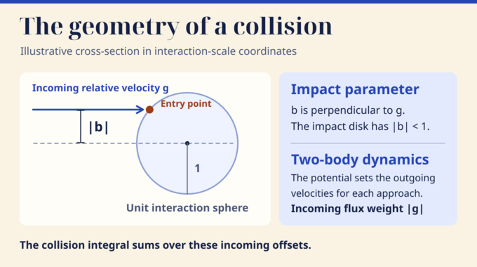
For incoming velocities and , let be their relative velocity. In interaction-scale coordinates, an impact parameter is the offset of the incoming line from the center, measured in the plane perpendicular to . The disk has unit radius. Integrating Newton’s two-body equations gives outgoing velocities and determined by , , and . Write for the gain product minus the loss product , at fixed time. The disk consists of with . The integral weights each offset by incoming flux. A pair with zero relative velocity contributes zero.
Slow escapes from a well complicate the scattering map. For bounded incoming speeds, the integral of residence time against incoming flux is finite because following each entry into the interaction ball sweeps out disjoint phase-space volume, and the relative speed stays bounded there. The flux of encounters lasting longer than a given time is therefore bounded by a constant divided by that time. Reversibility and flux preservation give the gain term in the same variables as the loss term. Integrating over incoming offsets automatically includes multiple offsets with the same deflection. Exceptional null-flux configurations can be set aside without requiring a globally regular angular cross-section.
8. Whole-Component Expansions Beyond Binary Collision Trees
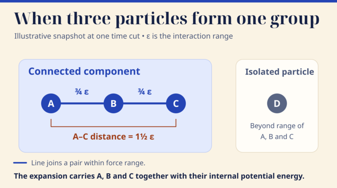
At a time cut, join particles within distance and keep each connected component, called a polymer in the paper, intact. If A is near B and B is near C, then A, B, and C form one component even when A and C exert no force on each other. The expansion carries the group’s actual internal dynamics and potential energy together.
Working backward through a fine cell, additional labels enter when needed to determine the displayed trajectories. Inclusion-exclusion over successive generations writes the result using exact subsystem flows and contact indicators. Some indicators record geometric contact between trajectories evolved independently in a signed term. Their role is algebraic. Keeping the true force groups intact allows stability to control their energy even when several internal encounters overlap.
9. Layered Centering and the Recovery of Molecular Chaos
The fine cells organize contact histories. Above them, a fixed number of coarser layers, each of length , gives places to compare with the kinetic solution. At each cut the proof centers only isolated single-particle slots. In the signed sum, a genuinely independent family cancels with its kinetic reference if its displayed paths, including detached paths, stay separated as required. A family with an extra contact can survive that subtraction, so its earlier history is carried into the next expansion. For a surviving centered root, the argument traces a chain back to an initial correlation, a small error in the local kinetic approximation, or a marked encounter history. The first two have small input bounds. The third needs geometry.
For a history with labels, the Gaussian weight comes from the velocities at the sources of those labels. Energy conservation through the cells and stability for intact departing groups control velocities at later cuts using the same budget. After accounting for the top roots, repeated velocity factors can cost up to , while ordered time integrals supply a layer-length factor for each addition. The resulting small base in the ordinary-history estimate scales like for a constant . Choosing sufficiently many layers makes large ordinary histories summable.
10. Causal Exposure of Recollisions and Complex Interaction Histories
A translation chart moves one group as a unit until a specified particle pair first meets. It replaces a relative translation by the contact time and surface direction. The spatial Jacobian contains times the normal relative speed, so the activity cancels the small area factor for an ordinary addition. Separate volume estimates handle crowded configurations and several additions in one fine cell.
After discarding parameter and crowding exceptions, histories with defects affecting a positive fraction of particle lives yield many disjoint terminal trees of bounded size in the time-ordered addition graph. Their fresh parameters include rotations of the incoming scattering data. Away from a small exceptional set, a genuine encounter gives nonzero velocity increments in both output branches relative to the old parent velocity. A required extra contact means a path controlled by the fresh direction must enter a thin spatial tube around a path already determined. The exposure order keeps that path independent of the parameter being tested, allowing the proof to multiply the small factors.
11. From Finite Particle Histories to the Boltzmann Equation
Large completed histories are exponentially suppressed by the combination of summability and rarity estimates. A separate problem is showing that stopping the expansion does little harm to the actual particle process. The proof chooses thresholds backward, making errors from earlier layers small enough to survive later amplification. It proves the bounds forward in time. A first violation produces a finite contact witness, and estimating that witness uses only remainders from strictly earlier layers. The resulting probability bound then controls the current stopping error. The forward induction also controls the finite mismatch created when the reference expansion uses a different selection from the stopped physical expansion.
With the cutoffs removed, the proof first obtains factorization for separated, externally isolated configurations. Since particle number is conserved, the total rescaled factorial mass stays equal to its initial value, which tends to one. The separated contribution already tends to mass one, so the omitted mass, including close configurations, vanishes. The first two marginals then control the mean and second moment of a rescaled empirical sum. Corollary B gives convergence in probability with a bound uniform over deterministic observation times. A pathwise maximum would require a different estimate.
12. What the Proof Means for Hilbert’s Sixth Problem and What Remains Open
The result extends regular-interval kinetic convergence from hard-sphere dynamics to a class of finite-duration forces that can attract. Its scope is a dilute gas in three-dimensional Euclidean space, with a fixed finite-range radial potential and the specified pair-excluded initial law. Applying it on a given time interval requires a classical Boltzmann solution with the stated bounds. The paper establishes the particle-to-kinetic step and leaves unconditional global existence and the separate passage to fluid equations outside its theorem.
The central lesson is that the Boltzmann equation can emerge even when the microscopic model permits interacting groups and repeated contacts. The proof accounts for those histories and shows that their extra correlations carry vanishing weight in the distributions the equation describes. Follow Binary Verse AI for more research explainers on the mathematical foundations of physics, including the Navier–Stokes problem and the Yang–Mills existence problem.
What is the Boltzmann equation used for?
The Boltzmann equation describes how particle distributions evolve through motion and collisions. It is fundamental to kinetic theory, nonequilibrium statistical mechanics, and the study of gas transport phenomena, including viscosity, diffusion, and thermal conductivity.
Can the Boltzmann equation be derived from Newton’s laws?
Yes. Earlier results established rigorous derivations under particular interaction and time assumptions. OpenAI’s 2026 preprint extends the derivation to stable, finite-range radial potentials throughout finite intervals on which the classical Boltzmann solution satisfies the required regularity and uniform Gaussian bound.
What is the Boltzmann–Grad limit?
It is a dilute-gas scaling in which the interaction range shrinks while the collision frequency stays of order one. In the three-dimensional grand-canonical model used in the proof, the particle activity is ε⁻², where ε is the interaction range.
What is molecular chaos in the Boltzmann equation?
Molecular chaos refers to the statistical independence used to describe particles entering collisions. Microscopic encounters can generate correlations. Under the theorem’s assumptions, the proof shows that every fixed-order rescaled factorial marginal becomes a product of one-particle densities in the limit.
What makes OpenAI’s Boltzmann equation proof different?
The proof accommodates attractive interactions, finite-duration encounters, recollisions, and clusters that form during the evolution. It combines whole-component expansions, layered centering, a common energy estimate, and causal exposure to establish convergence throughout regular kinetic intervals.
Does OpenAI’s proof solve Hilbert’s sixth problem?
It advances the kinetic part of Hilbert’s sixth problem by rigorously linking Newtonian dynamics to the Boltzmann equation for stable, finite-range radial interactions on regular kinetic intervals. Unconditional global existence of the kinetic solution and the broader mathematical foundations of physics remain outside the theorem’s scope.