
OpenAI’s Yang–Mills existence proof starts with matrices on the edges of a four-dimensional grid and ends with local quantum fields on continuous spacetime. The Yang–Mills Working Group’s November 10 assessment concludes that the Lean submission constructs relativistic pure Yang–Mills theories satisfying the specified Wightman axioms for compact matrix gauge groups with a nonabelian simple Lie algebra. The proof removes the lattice cutoff at fixed physical volume, extracts an infinite-volume limit, and reconstructs a quantum field theory in each pure phase. The positive mass gap and uniqueness of the infinite-volume limit remain open.
Table of Contents
01. What OpenAI’s Yang–Mills Existence Proof Actually Establishes
The construction realizes local gauge-invariant observables as quantum fields whose vacuum correlations come from the Wilson lattice law. The working group’s assessment supplies the theorem numbering used here and evaluates the October 28 Lean submission independently of OpenAI’s separate informal manuscript.
| Aspect | Finding or Status |
|---|---|
| Gauge group | A closed subgroup of a unitary matrix group with a nonabelian simple real Lie algebra. |
| Ultraviolet limit | Renormalized correlations at fixed physical volume converge along the entire chosen spacing sequence. |
| Infinite volume | A common subsequence yields all separated-point correlations at once. Uniqueness across subsequences remains open. |
| Quantum fields | Each pure phase yields a relativistic Wightman theory with a unique vacuum in that representation. |
| Short distances | A nonzero trace law, leading asymptotic freedom, and an operator product expansion with a controlled remainder. |
| Mass gap | A strictly positive spectral gap above the vacuum remains unproved. |
The OpenAI Yang–Mills proof concerns pure gauge theory, with gauge-field dynamics and no matter fields. The working group’s criterion for quantum Yang–Mills existence allows multiple candidate limits and phases. Selecting a vacuum for the full infinite-volume limit remains a separate question.
02. The Original Problem of Constructing Quantum Yang–Mills Theory in Four Dimensions
A gauge field is a connection . Its components specify how to compare internal degrees of freedom at neighboring points. They take values in the Lie algebra of the gauge group . The curvature measures the infinitesimal effect of transport around a loop. For matrix-valued fields the brackets denote the commutator, and the index runs over four Euclidean coordinates.
The commutator couples the components of the connection in the nonabelian theory. The formal Euclidean path integral weights configurations by the exponential of minus the integrated squared curvature, with a coefficient set by the coupling. The construction obtains continuum correlations through limits of finite-dimensional integrals.
Jaffe and Witten’s problem statement asks for a nontrivial quantum field theory with gauge-invariant local fields, the required short-distance behavior, and a positive mass gap. The Wightman framework makes the existence question precise through positive energy, covariance under spacetime transformations, commutativity at spacelike separation, and a vacuum from which field operators generate a dense set of states. Smearing the fields against smooth test functions makes their distributional meaning precise.
03. Why Earlier Mathematical Methods Could Not Complete the Construction
Perturbative renormalization organizes the divergences that appear at arbitrarily short distances order by order in the coupling. That organization leaves the problem of controlling actual correlations as the cutoff is removed. A finite lattice provides genuine integrals and an ultraviolet cutoff, but its spacing and preferred axes are built into the regulator. A continuum proof must recover full spacetime symmetry and keep local observables under control as the number of lattice degrees of freedom grows.
Balaban’s lattice renormalization program supplied a multiscale approach to ultraviolet control. The new argument follows that approach and adds machinery for comparing renormalized correlations at different cutoffs, then carrying them through to an infinite-volume reconstruction. This requires estimates on inserted local observables as well as on the effective action that determines their expectations. The action describes the law at a given scale. Insertions specify the observables whose joint correlations must survive the change of scale.
04. Starting With Wilson Lattice Gauge Theory and Local Observables
The lattice is a periodic four-dimensional box. An oriented edge carries a matrix , and reversing the edge replaces the matrix by its inverse. A plaquette is an elementary square. The ordered product around it transforms by conjugation under a gauge change, so its trace is gauge invariant. In the assessment’s normalization, the Wilson action sums the following weight once per positively oriented plaquette, with the matrix size.
The probability law weights the product of normalized Haar measures on the edge variables by the exponential of minus this sum times the inverse squared bare coupling, then normalizes the result. For a worked example, take lattice links obtained by parallel transport of a smooth connection. With spacing , the leading nonidentity term in the plaquette matrix is . The real trace removes the linear contribution, and the first curvature term in the plaquette weight is of order four.
This example identifies the classical observable encoded by the plaquette. The proof uses symmetry-adapted lattice polynomials as representatives and makes renormalized insertions by mixing labels of bounded degree with cutoff-dependent coefficients. Curvature has degree two, each covariant derivative adds one, and products add degrees. The local field spaces identify combinations of labels that vanish in correlations. Each phase retains the same spaces of null combinations, so passage to a phase preserves this local field content.
05. The Renormalization-Group Argument That Establishes the Continuum Limit
Theorem 4.1 fixes a physical side length , where indexes the chosen volumes, and uses a specified sequence of spacings tending to zero. The Wilson coefficient grows logarithmically in , with leading coefficient uniformly in . Here is the Lie algebra’s Casimir constant in the assessment’s normalization. The corresponding bare coupling shrinks as the grid is refined.
Renormalization-group blocking integrates out fluctuations at finer scales and transfers their effects into a coarser action. The proof explicitly tracks the marginal terms, whose influence persists under power counting, and propagates bounds on irrelevant terms, whose contributions are suppressed at coarser scales. Its gauge fixing preserves discrete lattice symmetries. With the insertions normalized through these transformations, comparisons of sufficiently fine cutoffs make the smeared correlations Cauchy.
For a label list and a smooth compactly supported joint test function inside the box and away from coincident insertion points, write for the smeared lattice correlation. The limit is represented by a smooth kernel away from coincidences modulo the box period.
The factor of lattice cell volume in the smearing is the Riemann-sum weight for each insertion. A single joint test function can probe how several insertions move together. The limit holds for the full chosen spacing sequence at each fixed volume. Universality under arbitrary choices of lattice spacings remains open.
06. From Finite Lattices to Infinite Volume Through Compactness
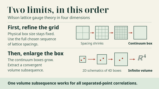
Theorem 5.1 expands the physical box after taking the fixed-volume continuum limit. Fix a compact set of point configurations with all insertions distinct. For sufficiently large boxes the correlation kernels are uniformly bounded there and share a modulus of continuity. Moving the points by a small distance changes the correlations by an amount bounded independently of the volume. Reflection positivity, chessboard estimates, transfer-operator methods, and Cauchy estimates contribute to these bounds.
Arzelà–Ascoli compactness yields convergent refinements on such compact sets. A common extraction works for every finite list of local labels and every allowed test function, so all the correlations belong to one limiting theory. The Wilson family and its normalization are fixed before choosing the order of volume extraction. Every strictly increasing order of the chosen volume indices admits such a refinement. Whether all refinements agree is an additional infrared question.
07. Phase Decomposition and Osterwalder–Schrader Reconstruction
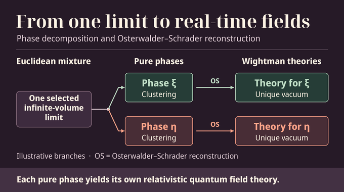
Fix one infinite-volume limit and call its correlations . Reflection positivity pairs a positive-Euclidean-time field expression with its time-reflected adjoint and gives a nonnegative quadratic form. Removing null vectors and completing yields a Hilbert space. Clustering, the factorization of distant groups of observables, is established for the component theories extracted from the mixture.
The proof compresses time-translated field words to the vacuum subspace and uses the resulting commutative operator algebra to decompose the mixture. The characters of that algebra index the components, is their compact space, and is a probability measure on it. For the same list of labels and test function, the correlations obey
A mixture can retain correlations between far-separated experiments if both are influenced by the same phase. Each component clusters and has its own unique vacuum in the reconstructed representation. Under Theorem 6.1, Osterwalder–Schrader reconstruction analytically continues the Euclidean correlations, taking distributional boundary values to obtain real-time Wightman functions. Those functions define the smeared fields on a common dense domain, with positive energy, Poincaré covariance, and local commutativity. Products of smeared fields acting on the vacuum generate a dense set of states. The phase-by-phase statement leaves equality between components unresolved.
08. Recovering Spacetime Symmetry Through the Stress Tensor and Ward Identities
The grid preserves coordinate permutations and sign changes. Full Euclidean invariance takes further work. The proof preserves discrete symmetries in gauge fixing, establishes local Ward identities from a conserved stress tensor, and uses reflection positivity in orthogonal planes to control stress flux at infinity.
The tensor is selected from a one-dimensional real space of symmetric, conserved, mixture-centered tensor labels of degree at most four with the required lattice transformation law. The translation Ward identity fixes its normalization. Let be the insertion to translate and let stand for the other insertions, held fixed. Write for their Euclidean correlation in phase . Choose a smooth compactly supported window equal to one near and zero near the other insertions. The identity reads
The gradient lives away from all insertions, so the integral tests separated points. The identity fixes the sign and coefficient of the local translation generated by stress flux.
09. Proving Nontriviality Through the Trace Anomaly and Asymptotic Freedom
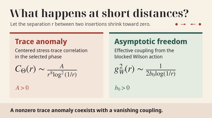
In the selected phase , let be the trace of the stress tensor with its vacuum expectation subtracted. Write for the Euclidean time unit vector and for the separation in the construction’s fixed units. Theorem 7.1 gives a positive leading amplitude for the centered two-point function.
The classical stress tensor in four dimensions is traceless. The nonzero quantum trace correlation is a trace anomaly produced by renormalization. Its leading coefficient agrees with the perturbative prediction in the same normalization. The inverse-square logarithm also rules out the finite free-field kernel descriptions specified in the assessment. The exclusion covers suitable polynomial observables built from finitely many free masses, with more general Gaussian composite descriptions outside its scope.
Theorem 7.2 defines an effective coupling from the blocked Wilson action and gives its leading short-distance running. Let . For any selected infinite-volume limit, the positive effective coupling satisfies
A second coupling defined from separated continuum correlations is asymptotic to . The vanishing coupling is asymptotic freedom. Rescaled stress-tensor correlations of the mixture approach those of independent Maxwell fields along a common short-distance sequence. The trace and coupling laws hold as tends to zero without that short-distance subsequence restriction.
10. The Operator Product Expansion and Its Short-Distance Predictions
Bring several insertions toward the origin while keeping other observables at fixed nonzero positions. The operator product expansion replaces that cluster inside a correlation by a sum of local fields at the origin. Each retained field has degree at most , the truncation degree. The coefficients depend on the collapsing insertions and are common across the mixture and its phases. Whether they agree across different infinite-volume limits remains open.
If the collapsing insertions have total degree , the remainder in the mixture or phase satisfies the following bound for every and sufficiently small positive , uniformly across phases and on fixed compact sets of separated configurations.
For two degree-four insertions truncated at degree eight, the exponent is . Choosing gives a vanishing absolute remainder for those fixed data. The cutoff limits the degrees of the retained fields. An order-by-order comparison of the coefficients with perturbation theory remains open. The proof also handles nested clusters under additional separation and scale conditions.
The submission constructs extensions across collisions. Terms supported on coincident configurations are invisible to separated-point tests, and uniqueness, full OS axioms, and lattice convergence for those extensions remain unproved. These extensions concern Euclidean correlators. The reconstruction separately gives real-time Wightman distributions on unrestricted Schwartz test functions.
11. What the Yang–Mills Existence Proof Resolves and What Remains Open
The mass-gap question asks whether the spectrum of the nonnegative Hamiltonian has an interval above the vacuum energy with no excitations. With the vacuum energy set to zero, a positive gap would require
Clustering supplies factorization at large separation. A gap calls for stronger infrared control, including exponential decay of appropriate correlations. The proof leaves the gap, uniqueness across volume subsequences, and continuum Wilson loop observables and their area law open. The spectral-gap problem in two-dimensional lattice systems and the Laughlin spectral-gap conjecture illustrate how the model and the operator determine the precise gap question. Even within a fixed lattice model, as in the quantum Heisenberg ferromagnet, the large-volume behavior calls for estimates specific to that model.
The working group reports a clean Lean rebuild, kernel and axiom audits, and Comparator checks against fixed specifications. The public theorem in Solution.lean calls the stronger construction theorem. The submitted kernel replay verifier checks dependencies of principal results. The group’s independent review package checks a stronger target tying the lattice law, limits, phase, and reconstructed fields to a common construction. One check follows a nonzero smeared trace correlation through both limits using the same test function and centering at every cutoff and volume. A separate comparison with earlier OS definitions covers the selected phase’s centered stress trace. Human review of the proof and definitions is ongoing. Our coverage of Fermat’s Last Theorem in Lean, the formalized Navier–Stokes result, and Anthropic’s formalized percolation theorem offers further examples of reading formal theorems by their precise scope.
The Yang–Mills existence proof gives the infrared questions a concrete object to study in the relativistic continuum theories tied to Wilson’s lattice model. Their leading short-distance laws give concrete tests of the Yang–Mills identification. Establishing how those theories behave across arbitrarily large distances is the next mathematical task. Follow Binary Verse AI for research explainers that trace the claim from the source to the theorem, including our coverage of OpenAI’s Astra mathematical proofs.
What does Yang–Mills existence mean?
It means rigorously constructing a four-dimensional quantum gauge theory with well-defined local observables and the properties required of a relativistic quantum field theory. In this construction, the observables are defined through correlation functions and reconstructed quantum fields.
What exactly did OpenAI’s Yang–Mills proof establish?
The Lean submission constructs continuum theories from four-dimensional Wilson lattice gauge theory for compact matrix gauge groups with a nonabelian simple Lie algebra. Each pure phase of a chosen infinite-volume limit reconstructs to a relativistic quantum field theory satisfying the specified Wightman axioms.
How did OpenAI overcome the continuum-limit difficulty?
The proof uses renormalization-group transformations to control correlations of renormalized lattice observables as the ultraviolet cutoff is removed. At fixed physical volume, convergence holds along the full spacing sequence chosen by the construction. The subsequent infinite-volume limit is taken along a subsequence.
Why is Osterwalder–Schrader reconstruction essential?
It turns Euclidean correlation functions into relativistic quantum fields. The proof decomposes a chosen infinite-volume limit into components that satisfy clustering, then reconstructs a Wightman theory with a unique vacuum in each component representation.
Does OpenAI’s proof establish a positive Yang–Mills mass gap?
No. The working group concludes that the construction satisfies its stated existence criterion. A positive mass gap and uniqueness across infinite-volume subsequences remain unproved.
Does the proof establish a unique quantum vacuum?
Each reconstructed component has a unique vacuum in its representation. Agreement of the components and uniqueness of the infinite-volume limit remain open.
How was OpenAI’s Lean proof independently validated?
The Yang–Mills Working Group reports a clean Lean rebuild, kernel and axiom audits, and Comparator checks against fixed specifications. It also used independent Lean comparisons to test how the formal statements capture the intended construction. The group describes its human review as extensive and still incomplete.