
A zero of order two vanishes from a divisor record taken modulo two. Lose enough zeros and poles this way, and it seems impossible to recover the field that produced them. OpenAI’s Milnor K-Theory manuscript shows why the loss can be overcome. For finitely generated function fields of transcendence degree at least two over algebraically closed constants of characteristic different from the chosen prime ℓ, the first two mod-ℓ Milnor K-groups and their full product determine the perfect closure and its constant field. The turning point is a five-fiber argument. A curve map can hide zeros by making them highly ramified, but a curve of bounded genus has only so much ramification to spend.
Table of Contents
1. What OpenAI’s Mod-ℓ Milnor K-Theory Reconstruction Theorem Proves
Theorem 1.1 of the October 5 manuscript is an isomorphism theorem. If a linear bijection on degree one respects the product relations, a constant-preserving isomorphism induces it up to the stated scalar. Here denotes the perfect closure of a field . The constants themselves are recovered up to isomorphism. In characteristic zero the perfect closure is the original field.
2. The Bogomolov–Pop Problem: What Earlier Reconstruction Theorems Could Not Establish
Birational anabelian geometry asks how much of a function field can be read from its Galois-theoretic invariants. Bogomolov proposed using a pro-ℓ quotient in which commutators are central. Bogomolov and Tschinkel proved reconstruction over algebraic closures of finite fields, first for surfaces and then in higher dimensions. Pop independently completed reconstruction over those constants and obtained a result for more general algebraically closed constants using pro-ℓ data equipped with divisorial inertia in relative transcendence degree greater than two.
For the finite-coefficient problem, Adam Topaz’s mod-ℓ theorem worked in relative transcendence degree at least five and took the rational subgroups as additional input. These subgroups are the images of multiplicative groups of relatively algebraically closed rational one-variable subfields. The new manuscript recovers the relevant rational subfields from the product and uses their point values to work from dimension two. OpenAI’s release attributes the results to an internal frontier model. The manuscript documents the proof’s logical steps, and the release describes the model contribution at the collection level.
3. Why Two Milnor K-Groups and the Steinberg Product Contain Field Information
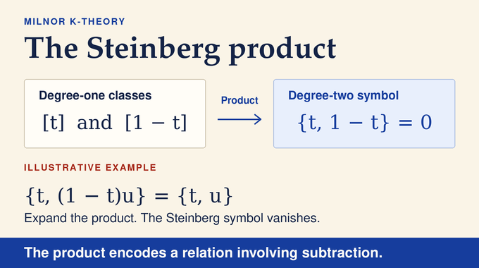
For a field , put and write for the class of a nonzero element . Degree one is . The group law is written additively, so . The mod-ℓ Milnor K2 group is the tensor square of over modulo the subspace spanned by for . The product sends a pair to its symbol . The vanishing of is the Steinberg relation.
For an indeterminate in and any , bilinearity gives an illustrative calculation.
Compatibility means that carries onto . It therefore induces the unique degree-two isomorphism that intertwines the products. The product makes subtraction visible through linear relations.
4. The Six-Stage Proof Roadmap: From Multiplicative Data to Field Operations
- Detect valuations. Find pairs of characters whose evaluations agree in a particular way on every Steinberg relation. Large spaces of such characters expose the valuations that organize the proof.
- Find the points of residual curves. Follow chains of valuations until one geometric variable remains. Recognize the point orders on useful residual curves and use their kernels to read genus.
- Bound the visible divisor support. Use five fixed values of one rational function to bound the separable degree on a test curve. This controls the support of every remaining member of its pencil.
- Recover curve subfields. Collect infinitely many divisors of bounded degree into a family. One parameter curve gives a candidate one-variable field, and exact descent brings it back to the target field.
- Identify rational coordinates. Recognize divisors trivial on constants and recover rational subfields whose projective points can all be detected by these divisors.
- Recover arithmetic and prove uniqueness. Compare simultaneous coordinate values, use additive triples to align the constants, and extend the resulting correspondence to the perfect closures. Then account for scalar and Frobenius ambiguity.
5. Recovering Valuations from Alternating Characters
A character is a homomorphism , or equivalently a linear functional on . Two characters are alternating when for every . Their determinant functional then vanishes on , so a compatible isomorphism preserves alternation on the dual spaces. The input supplies no named valuation rings.
Section 2 uses alternating-pair valuation theory to prove that the largest dimension of an alternating space equals the relative transcendence degree . A one-dimensional intersection of two -dimensional alternating spaces is the inertia line of a unique quasi-divisorial valuation , and every such valuation arises this way. Its relative value group is cyclic and its residue field has relative transcendence degree . The inertia consists of characters killing valuation units.
The decomposition space consists of characters killing principal units, and is exactly the space alternating with a nonzero generator of . Passing to gives the residue-field character space. Repeating this procedure produces flags that end at one-variable residue fields. Quasi-divisors may act nontrivially on constants, allowing the residue characteristic to change.
6. How Residual Curves Reveal Point Orders and Constant Fields
On the smooth projective curve of a one-variable residue field, a point defines the character . Pop’s density theorem helps construct an intrinsic family of candidate inertia lines containing the point lines. Further reduction of the constants can also contribute lines, so Section 3 tests the relations among candidates.
Every rational function has finitely many zeros and poles, so its point orders can be summed. Their sum is zero because a principal divisor has degree zero. Any relation factors through the divisor class group, whose degree-zero part is ℓ-divisible. Thus constant coefficient families give the entire kernel of the summation map. If the residue constants are algebraic over a finite field, the candidates are exactly the point lines. Otherwise, reduction of the constants contributes extra lines.
The relation among the actual point lines has zero coefficients on those extras, so it fails the requirement of a unique relation with every coefficient nonzero. The intrinsic test recognizes the first situation and matches the complete point families. In residue characteristic different from ℓ, the common kernel of all the point orders on the multiplicative classes has dimension , where is the genus, by the ℓ-torsion of the Jacobian.
7. The Five-Fiber Argument: Controlling the Divisors Lost Modulo ℓ
Fix a normal projective model of . The support degree of a class is the sum of the degrees of the prime divisors on where its order is nonzero modulo ℓ. Section 4 constructs a residual curve for each finite independent list of classes. General hyperplane sections meet the relevant divisors transversely and preserve independence via an integral cover obtained by adjoining ℓ-th roots. Specialization retains these properties over constants algebraic over a finite field. The number of visible point orders equals the support degree, and the genus is bounded by , determined by the embedded model.
For the pencil of classes , choose five fixed anchors from the cofinite independent subfamily and test them together with one further member. After transporting across and normalizing the residues on the side, the six classes come from a single residual pencil. In characteristic zero, three anchors whose differences include and ℓ ensure that the residue characteristic differs from ℓ. Removing the purely inseparable power gives a separable map to the projective line of degree . The removed power multiplies orders by a unit modulo ℓ.
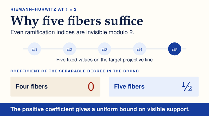
Let be the support degree on of anchor . In its fiber, at most points have ramification index visible modulo ℓ. Every other point uses at least ℓ of the total fiber degree, leaving at most points in all. Each fiber contributes at least its degree minus its number of points to the different, the ramification term in Riemann–Hurwitz. Summing across five disjoint fibers gives the manuscript’s inequality.
At , the coefficient is . Four fibers would give zero in this estimate, and for larger primes the five-fiber coefficient grows. The test member has zeros and poles in two fibers, so at most visible orders. The right side stays fixed as the test member varies. Including the finitely many omitted parameters gives a uniform support-degree bound for the entire pencil.
8. From Bounded Divisors to Curve Subfields: The Incidence Argument
A curve subfield is relatively algebraically closed in and has transcendence degree one over . Fix . The supports of contain infinitely many distinct divisors of bounded degree. Otherwise the pencil’s infinite-dimensional span would have to fit into finitely many order coordinates plus a finite-dimensional kernel. For any class in , the valuation correspondence forces its representative to have ℓ-th-power residue along all but finitely many of these divisors. On the source curve, a valuation detected by a pencil member leaves only constant residues. Its inertia and decomposition characters therefore have the same restriction image on .
Bounded degree puts the divisors in a finite-type parameter space. On an integral parameter curve, the incidence variety pairs each divisor with the points lying on it. Its function field is finite over and is the compositum , where is the parameter curve’s function field. For each class, its Kummer cover splits generically after a finite parameter change. Normality extends that splitting over the smooth locus where the representative is a unit. So the same parameter curve works for every class, even though the finite change can depend on the class.
In a finite normal overfield, the relative algebraic closure of the parameter field is preserved by automorphisms over because distinct curve subfields have only a finite-dimensional intersection of their mod-ℓ images. Intersecting with gives a curve subfield there. The compositum identity lets the root test descend exactly, avoiding a norm that could kill a class modulo ℓ. Applying the argument in reverse completes Theorem 5.4. Every matches a unique curve subfield of with .
9. Recovering True Divisors and Rational Subfields
A true divisor is trivial on the constants. Section 6 recognizes it by finding a curve subfield on which the kernel of evaluation against its decomposition space is finite-dimensional. A true divisor admits such a subfield because a unit can have transcendental residue. A valuation nontrivial on constants instead supplies infinitely many independent principal-unit classes on every curve subfield.
At a smooth point, choose vanishing functions with independent linear terms. Blowing up the point makes the residue of a rational coordinate on the exceptional divisor, proving that its rational subfield is relatively algebraically closed. Each local divisor detects the value with order one, and detects infinity. The paper calls such fully detected rational subfields good. The point-line relations identify them and match their projective points. Good functions generate the field because any nonzero function can be written as the ratio of two good functions.
10. Reconstructing Addition from Simultaneous Values
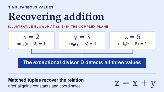
A blowup at a general smooth point detects the values of several good functions at once. Each function minus its value has order one on the exceptional divisor, so no coordinate disappears modulo ℓ. The matching divisor gives simultaneous values on the target, transporting a dense set of tuples in each direction between the varieties of algebraic relations.
The paper applies this to with algebraically independent and all three good. For example, the source relation transports to a perfect rational expression in the two target coordinates. One-variable slices reveal translations and dilations. Their conjugation law recovers multiplication on constants from the slopes of dilations acting on translations. The two-variable law proves that the resulting embedding is onto. A common partner for pairs of good functions aligns their point maps, up to projective transformations and Frobenius powers, with a single constant-field isomorphism. After these adjustments, taking Zariski closures removes the finite exceptional coordinate values and transports every polynomial relation. The adjusted generators then give an isomorphism of perfect closures.
11. Why the Reconstruction Is Unique: Perfect Closure, Scalars and Frobenius
Compare the constructed field isomorphism with the original compatible map. The resulting linear automorphism preserves the degree-one image of each good subfield. These images distinguish true divisors, so the dual automorphism fixes every point line on each good projective line. The single relation among point orders forces a common scalar on that line. A blowup whose inertia is visible on two good subfields forces their scalars to agree. The classes of good functions span degree one, yielding a global , and bilinearity gives on degree two.
In characteristic , purely inseparable extensions are invisible because taking -powers acts by invertible scalars modulo ℓ. Frobenius itself acts by on degree one. Conversely, a scalar action fixes each unordered pair of points on every good line. The induced point permutation is therefore trivial, forcing the field automorphism to be a Frobenius power or the identity in characteristic zero. At the degree-one scalar is trivial, while positive-characteristic Frobenius ambiguity remains. The theorem requires relative transcendence degree at least two and ℓ away from the characteristic. The release’s Lean record covers injectivity for the companion pro-ℓ Galois theorem, a narrower uniqueness result with ℓ-adic unit scaling.
The decisive move in this Milnor K-Theory proof is to turn information lost at individual divisors into a global bound that survives reduction. That bound recovers enough curves to make simultaneous values, and ultimately addition, visible. Follow Binary Verse AI for more paper-first coverage of AI-generated proofs, including the Zariski cancellation problem in algebraic geometry and the Deligne–Drinfeld conjecture in the Grothendieck–Teichmüller program.
Can Milnor K-theory reconstruct a function field?
Yes. For a finitely generated function field of transcendence degree at least two over algebraically closed constants of characteristic different from ℓ, the first two mod-ℓ Milnor K-groups and their full bilinear product determine the perfect closure and its constant field.
Why are both and necessary?
Degree one records multiplicative classes. The paper also uses the degree-two product, whose kernel contains the Steinberg relations. These relations let the proof detect alternating characters and recover valuation data.
What makes OpenAI’s proof different from earlier Bogomolov–Pop reconstruction results?
It recovers the required rational subfields from the mod-ℓ product itself. It applies in relative transcendence degree at least two over any algebraically closed constant field of characteristic different from ℓ.
Why does the proof use five fibers and Riemann–Hurwitz?
Five fixed fibers give a positive coefficient in the Riemann–Hurwitz estimate for every prime ℓ. At it is . The estimate bounds the separable degree on a test curve and thereby gives a uniform bound on the visible divisor support of the pencil.
How can addition be reconstructed from multiplicative information?
The recovered rational subfields give corresponding projective point sets. Divisors detect several coordinate values at once, and the algebraic relations of additive triples align those point correspondences with field operations.
Why does the theorem reconstruct the perfect closure rather than necessarily the original field?
Purely inseparable extensions preserve these mod-ℓ groups and their product. In positive characteristic, Frobenius acts by a nonzero scalar on degree one, so the inducing field isomorphism is unique modulo Frobenius after allowing a single global nonzero mod-ℓ scalar.