

Imagine choosing network connections while an opponent already knows every value, every sample and every coin you will flip. Your decisions remain irreversible. OpenAI’s September 23, 2026 paper proves that a matroid prophet inequality survives this information imbalance: one independent sample per element suffices for a universal expected reward fraction of . The detailed proof establishes . These are theoretical guarantees, with no practical efficiency claim. The achievement is a constant independent of the matroid’s size and rank, even when the opponent chooses the arrival order after seeing the complete random seed.
Table of Contents
1. What Is a Matroid Prophet Inequality? The Original Problem
A matroid consists of a finite labeled ground set and a family of feasible, independent subsets. Independence is hereditary, and a smaller independent set can be augmented from a larger one. Rank is the largest independent subset size in . Online selection observes one label and value at a time, accepting or rejecting immediately. The offline prophet sees everything and maximizes the total feasible value:
| Feature | Verified Statement |
|---|---|
| Information | One independent sample per element, with no distribution descriptions |
| Feasibility | Any known finite labeled matroid |
| Adversary | Sees samples, online values and the entire seed |
| Expected Reward Fraction | stated, proved in Section 6 |
| Computation | Finite measurable rule, no polynomial-time guarantee |
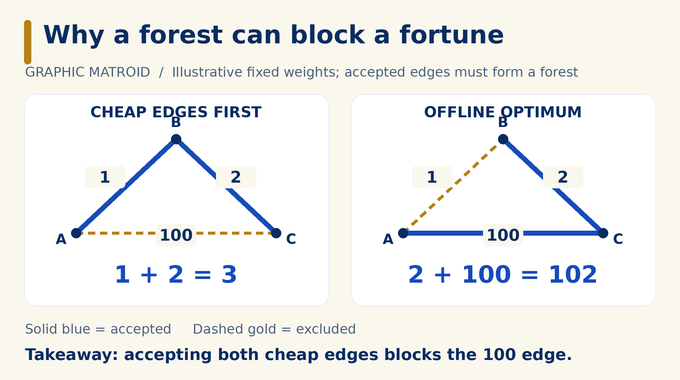
For a graphic matroid, labels are edges and independent sets are forests. In the triangle below, accepting both cheap edges earns 3 and blocks the remaining edge. The offline optimum earns 102. This deterministic example illustrates feasibility pressure, rather than a counterexample to the stochastic theorem.
2. Why Previous Prophet Inequalities Could Not Handle an Almighty Adversary
The title’s distinction concerns the information model. The classical known-distribution matroid guarantee is . As the paper explains, that adversary may adapt to revealed values, but does not see unseen values. Previous one-sample guarantees for general matroids incurred a doubly logarithmic rank loss. Earlier constant guarantees against an almighty adversary used sample budgets growing with the instance.
There is also a one-sample result with independence queries, cited in the paper, whose order is fixed independently of samples, values and coins. Thus neither “one sample” nor “constant competitive” alone identifies the new result. Their combination with full-seed order selection does.
This distinction resembles the need to specify an opponent’s powers in randomized online algorithms. A guarantee for each fixed order does not automatically survive an opponent choosing an order separately for every realized seed.
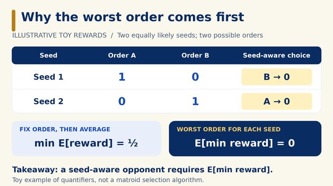
A two-order toy example makes the quantifiers concrete. Suppose a fair seed yields rewards 1 and 0 for two possible orders, with those rewards reversed under the other seed. Each fixed order has expected reward one half. An opponent observing the seed always picks the zero-reward order. The expected minimum is zero. This illustrates the logical gap, without asserting such a toy rule solves the selection problem.
3. OpenAI’s One-Sample Theorem: What the Proof Guarantees
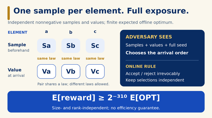
Theorem 1.1 assumes mutually independent nonnegative real variables , with each sample and corresponding online value sharing an arbitrary law . Different elements need not share distributions. The seed is independent of all these variables, and the expected offline optimum is finite.
Here is the accepted independent set. The inequality holds for every measurable arrival permutation depending on the matroid, distributions, samples, values and seed. The algorithm knows the labeled matroid and receives the sample vector, but lacks distribution descriptions and the future order.
The original research paper supplies the mathematical statement. OpenAI’s release announcement provides release context, rather than an additional theorem or performance benchmark. “One-sample matroid prophet inequality” means one sample per element, not one observation for the entire instance. The expectation averages the algorithm’s reward, so the bound is not promised separately for every realized value vector in the stochastic model.
4. The Hidden-Weight Reduction: Making the Worst Arrival Order Explicit
Proposition 2.1 starts with fixed hidden weights . A random mask reveals some weights and sacrifices those labels, forcing rejection. The target places the minimum inside the expectation:
Moving the minimum outside would let a different order look favorable under averaging, leaving the seed-aware opponent uncontrolled. Instead, each realized seed is evaluated against its worst permutation.
Lemma 2.2 glues sample coordinates on the revealed mask to online coordinates elsewhere:
Conditional on any seed, each chosen coordinate has law , independently across labels. This product law does not depend on the seed, so the glued vector is independent of it and distributed like . Simulating the hidden-weight rule then earns actual online values on accepted labels. Even unused samples known to the adversary cannot defeat the pointwise minimum over orders.
For one coordinate, suppose both independent copies equal 10 or 0 with equal probability. Choosing the sample copy through a seed-determined mask still gives either value with probability one half. Choosing the online copy does too. The crucial restriction is that the mask is selected independently of the weights, rather than by inspecting which copy is larger.
5. Geometric Weight Rounding, Candidate Selection, and Random Masks
Positive weights round down to , with and zero kept zero. The rounded optimum lies between and . A fair branch choice separates concentrated value from value distributed across many elements.
The maximum branch samples a fair mask and accepts the first unsacrificed positive nonloop beating all revealed labels in priority. It earns at least one quarter of the largest rounded nonloop weight in expectation against every order. The main branch uses four independent masks:
| Mask | Membership Probability | Purpose |
|---|---|---|
| Filters candidates using higher-priority span | ||
| Lists weight groups and supplies density data | ||
| Supplies guards | ||
| Thins online eligibility |
Labels in are revealed and sacrificed. Membership in alone reveals nothing. A candidate lies outside and outside the span of higher-priority labels. Lemma 3.1 retains expected optimum-comparison weight , while bounding total expected candidate weight by . Weight groups are listed only when hit by .
6. Density Expansions: How Sampled Values Build Matroid Flats
Closure contains exactly the labels whose addition does not increase rank. A flat equals its closure. Conditional rank is . For listed group , its density sample is . With , the expansion is the largest flat maximizing
The objective rewards sampled labels captured while charging rank. Supermodularity ensures a largest maximizer exists, and Lemma 3.2 proves the expansion is monotone in its base. For , the residual inequality is
Any further extension captures at most its rank cost times additional sampled labels. Lemma 3.5 strengthens this accounting across the whole path: one set of at most generators suffices. Charging each auxiliary time separately would repeatedly bill the same sampled structure. This is rank accounting, distinct from the geometric objectives in metric k-median optimization.
For a concrete density calculation, take a rank-one parallel class, where any single nonloop spans the class. Starting from the loop flat, capturing its entire density sample contributes its sample count minus the rank charge. If that count exceeds the charge, expansion improves the objective. Thus many sampled labels can justify consuming just one unit of rank.
7. Guarded Flat Paths: Why Greedy Selection Remains Feasible
Process listed groups from low to high weight. The nominal path expands the preceding group’s guarded flat. The guarded path additionally spans guard labels from the next nominal step. Consequently,
The integer is auxiliary path time, unrelated to arrival time. A fair parity chooses alternate endpoints, creating layers on the final guarded path. Within each layer, greedy selection accepts only labels independent over its earlier endpoint flat. Earlier layers lie entirely inside that base, so combining layerwise independent sets stays feasible under every arrival interleaving.
Eligibility also requires the appropriate nominal birth, a listed weight, test-mask membership and exclusion from sacrificed masks. Baseline births are discarded so the density map is already enabled at the earlier endpoint. This structural feasibility proof precedes reward analysis. As in scheduling under feasibility constraints or bin packing, counting attractive choices without checking their compatibility would miss the central difficulty.
8. Reverse Exposure: Protecting Valuable Elements From Lower-Weight Arrivals
Lower-weight arrivals can occupy rank before valuable candidates appear. Section 4 counts sampled comparison labels that remain outside a density expansion containing the earlier flat and all potential lower-weight test competitors. These are called safe samples.
Analyze guards backwards in auxiliary time, making nominal flats shrink. Each step queries previously untouched bits only. Conditional on the query transcript, untouched coordinates retain their independent Bernoulli laws. This is an analysis of initially drawn randomness, all visible to the adversary.
A disjoint-query certificate bound limits repeated survival certificates for an increasing event. It shows substantial exit mass occurs at steps with conditional exit probability at least . A hybrid transition replaces departing coordinates’ guard bits with independent test bits while retaining unqueried guards. Ordinary and hybrid exits yield a squared exit probability and imply safety. Lemma 4.3 concludes:
Here is the optimal rounded independent set minus , and counts safe sampled labels. As with sampling guarantees, the conditioning and preserved probability law are essential.
9. Marked Pivots: Recovering Rank From Sacrificed Samples
Safe sampled labels cannot be accepted because their information was purchased through rejection. Section 5 instead chooses unsacrificed rank witnesses in each layer, with total size . Unspanned labels form a residual contained entirely in . The density inequality gives
A large residual could therefore absorb the safe count. Bounding one fixed residual is insufficient: the paths and witnesses select it using the very masks being analyzed. The proof first constructs a uniform family containing every possible relevant residual.
Lemma 5.2 marks occurrences in a spanning sequence. A label’s pivot is the first occurrence after which it becomes spanned. With tested labels and at most movable occurrences, the number of pivot-mark vectors is bounded by
Greedy-basis counting supplies the first factor. Encoding last support members by dominating signed scores reduces the remaining possibilities to affine sign patterns. Crucially, no timeline-length factor appears. Two such encodings describe residuals, enabling a union bound before focal mask exposure. Lemma 5.1 then transfers safe counts to unsacrificed rank, with controlled error.
The same mechanism explains why counting all subsets would be wasteful. The residual may look arbitrary after mask exposure, but bounded generator and witness budgets constrain which subsets can arise. Marked pivots describe that dependence before the random mask is seen.
10. From Rank to Reward: Deriving the Final Competitive Ratio
Lemma 6.1 constructs a rank statistic independent of order that lower-bounds the number of accepted labels at least as heavy as group . Equivalently, that accepted count is at least for every permutation with all coins fixed.
Lemma 6.2 pays for later guarded expansions once. A common generator set bounds conditional-rank losses, whose sum telescopes across the path. Lemma 6.3 then averages the focal group’s independent test mask, preserving a factor of remaining rank. No chosen arrival order is conditioned upon.
Geometric levels convert cumulative accepted counts into reward. Higher-level costs are controlled by a geometric series. Small groups can be discarded when the largest rounded weight is small relative to , giving main-branch reward at least , where . Otherwise, the maximum branch covers the loss. Fair branch mixing and rounding give
The matroid prophet inequality competitive ratio leaves explicit slack. Both numbers are proved reward fractions, not measured success rates.
11. What OpenAI’s Proof Establishes and What Remains Unresolved
The result removes rank dependence under one-sample information and full-seed adversarial ordering. Its tiny constant is not a useful deployment target. The construction is finite and measurable, but establishes no polynomial running time or independence-oracle complexity bound. Improving efficiency and the guaranteed fraction remains open within this paper.
Corollary 7.1 also gives an order-oblivious secretary guarantee of : fixed weights precede randomness, a uniformly random prefix is observed and rejected, and the fully informed adversary may reorder the suffix. It cannot choose weights after seeing the seed or change the prefix law.
The published Lean scope document identifies formalized one-sample and hidden-vector statements, including prefix feasibility and full-seed order dependence. This article has not independently rebuilt the Lean project. Formal checking concerns encoded mathematics, while novelty and practical usefulness require separate assessment. That distinction also matters when reading complexity lower-bound results.
The lasting matroid prophet inequality lesson is that visible randomness can still support a universal expected guarantee when feasibility and losses are controlled uniformly over orders. Explore Binary Verse AI’s connected research explainers, and use the original statements to follow what each proof actually establishes.
What is a matroid prophet inequality?
A matroid prophet inequality compares the expected reward of an online algorithm making irrevocable selections with the expected optimum achievable after all values are known. Both must respect the same matroid independence constraints.
Does the proof require only one sample for the entire matroid?
No. The algorithm receives one independent sample for each element, drawn from the same distribution as that element’s eventual online value. It does not require knowledge of the distributions.
Must every element have the same probability distribution?
No. Different elements may follow different arbitrary nonnegative distributions. Each sample and its corresponding online value must have matching laws. All sample and online-value variables are mutually independent, and the seed is independent of them. The expected offline optimum must be finite.
What makes an almighty adversary different from an ordinary adversary?
An almighty adversary knows all samples, actual online values and the algorithm’s entire random seed before selecting the arrival permutation. The algorithm still has to decide online without knowing the future order.
Why does the proof obtain instead of the classical guarantee?
The classical matroid result assumes known distributions and a weaker adversarial information model. The new construction uses one sample per element against a fully informed ordering adversary and proves a smaller universal guarantee. Its detailed argument establishes , while Theorem 1.1 states .
Does OpenAI’s proof provide a polynomial-time algorithm?
No polynomial-time implementation or independence-oracle complexity guarantee is established. The paper constructs a finite measurable online rule, so its principal achievement is mathematical feasibility rather than practical efficiency.
Has the matroid prophet inequality proof been formalized in Lean?
Yes. OpenAI’s published Lean scope document identifies formalizations of the one-sample guarantee and the supporting fixed-weight result. This article has not independently rebuilt that project. Formal verification of encoded statements is distinct from assessing novelty and practical usefulness.