

A dynamical system can require fresh geometric information at every step, even when its orbit lives inside one compact space. Can its associated algebra measure that same complexity exactly? The Phillips–Toms conjecture predicts that it can: the radius of comparison equals half the mean dimension. OpenAI’s September 25, 2026 paper proves this equality for every minimal homeomorphism of an infinite compact metrizable space, including infinite values. The crucial advance establishes the missing lower bound by turning algebraic comparison into a reduction in covering order. A sharp upper bound was already known. Together, they identify precisely how much dynamical dimension the crossed product retains.
Table of Contents
1. What the Phillips–Toms Conjecture Actually Predicts
The paper’s Theorem 1.1 concerns a homeomorphism . Minimality means every orbit is dense. The space must be infinite, compact and metrizable, but need not have finite covering dimension. With these assumptions, the theorem states:
Both sides take values in the extended nonnegative reals. Mean dimension measures topological complexity per iterate. Radius of comparison measures how large a gap between tracial size functions guarantees comparison of positive algebra elements.
| Item | Verified Scope |
|---|---|
| System | Minimal homeomorphism of an infinite compact metrizable space |
| Acting group | The integers |
| Exact relationship | Radius of comparison = one half of mean dimension |
| New contribution | Matching lower bound for every finite orbit cover |
| Topological input | Compression theorem imported from a companion paper |
| Endpoint values | Both zero and infinity are included |
The result belongs to OpenAI’s mathematical research release. The supplied PDF presents a mathematical proof, rather than a performance benchmark. It does not document a Lean formalization of this theorem. For a formal-proof example, see our Fermat’s Last Theorem in Lean coverage.
2. From Minimal Dynamics to Crossed Product C*-Algebras
The algebra combines continuous complex-valued functions on with a unitary representing one step of the dynamics. Products record how functions interact with their shifted versions. Completing these expressions in the appropriate operator norm produces the crossed product C*-algebra.
Write for this algebra. Related operator-algebra questions appear in our Naimark problem and free group factor isomorphism explainers.
This construction retains more than the collection of points in the space. It includes how the homeomorphism moves those points. An orbit representation makes this concrete: a function acts diagonally by its values along an orbit, while the implementing unitary shifts the orbit index.
Minimality and infinitude exclude periodic points. Otherwise a finite orbit would be a nonempty closed invariant subset, and minimality would force it to equal the infinite space. The resulting integer action is therefore free. The crossed product is simple and nuclear, and invariant probability measures supply tracial states. These properties allow the paper to connect orbit geometry with comparison and classification theory.
3. Mean Dimension: Measuring Complexity Along an Orbit
Start with a finite open cover , a finite collection of open sets covering . A refinement uses smaller sets, each contained in an original member. The order of a cover is its largest possible overlap minus one. The quantity is the least order among finite open refinements.
Observing successive iterates requires the orbit join:
Its members are intersections specifying which cover sets contain the first orbit positions. Define the rate for this cover:
Mean dimension is the supremum of these rates over all finite open covers.
Subadditivity guarantees each cover’s limit exists and is finite. Their supremum can be infinite. Mean topological dimension therefore measures sustained dimensional growth, rather than the dimension of one snapshot. Infinite covering dimension alone does not determine the answer. For another dynamical invariant, see our Shub entropy conjecture explainer.
For a simple overlap example, a cover in which at most three members meet has order at most two. Its refinement order might be smaller, because better choices of open sets can eliminate unnecessary overlaps. The proof must control this optimized quantity, not just count the sets in the original cover.
4. Radius of Comparison: When Traces Guarantee Comparison
Take positive elements and in finite matrix algebras over , allowing enlargement into compatible corners. Cuntz subequivalence, written , means that matrices can compress to approximate in norm. It generalizes the idea that one projection fits inside another.
For each normalized tracial state , the dimension function is:
Here is the unnormalized matrix trace. A finite nonnegative number is a comparison bound when:
The radius is the infimum of all such bounds, or infinity if there are none. For a positive matrix function , tracial dimension is its pointwise rank integrated against the corresponding invariant measure. A constant rank-three projection therefore has dimension function three. Replacing by a normalized matrix trace would change this scale and invalidate the stated gap convention. The theorem’s one-half constant uses the paper’s normalization throughout.
The inequality is strict and must hold for every normalized trace. An average gap for one invariant measure would not satisfy the definition. For related operator theory, see our Crouzeix conjecture explainer.
5. Why the Formula Contains Exactly One Half
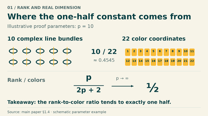
Complex bundle rank and real dimension supply the underlying scale. A complex line has real dimension two. But that observation alone does not prove the equality: the argument must preserve actual cover information while converting rank estimates into dimension savings.
For a positive integer , the construction uses a rank- bundle assembled from complex line bundles over a product of two-dimensional tori. On the cover side, it groups colors into a packet. Their normalized weights form a simplex of dimension , identified with a cube of the same dimension.
For example, ten complex lines correspond to twenty-two colors, giving the ratio 10/22, approximately 0.4545. Increasing the rank approaches one half. This is an illustration of the proof’s parameter arithmetic, not a computed dynamical example. The limiting argument leaves room for tower errors and rounding before recovering the exact constant.
6. The Previous Results and the Lower Bound They Could Not Establish
The sharp upper estimate predates this paper.
| Result | Contribution |
|---|---|
| Phillips | Radius at most one plus thirty-six times mean dimension |
| Elliott–Niu | The zero-mean-dimension case |
| Niu | Radius at most one half of mean dimension |
| Hirshberg–Phillips | Lower bounds using mean cohomological independence |
| OpenAI, Theorem 5.1 | Every cover rate satisfies for every finite comparison bound |
Phillips’s earlier upper-bound argument established finiteness under finite mean dimension. Niu’s optimal upper-bound theorem supplied the conjectured constant. Earlier lower bounds detected translated cohomology classes and their nonvanishing products. Those hypotheses did not recover arbitrary orbit-cover rates. What remained was to prove that radius is at least half the mean dimension. The new proof obtains this inequality without imposing cohomological independence or finite dimensionality.
7. The OpenAI Proof Begins with a Contradiction
Fix a finite comparison bound and a finite open cover . Suppose . The goal is to build a refinement whose long-term order is smaller than the rate defining that same cover. Such a refinement would contradict the definition of .
Choose a long orbit window of length and a subordinate nerve whose dimension is the least refinement order for that window. A nerve is a simplicial complex recording which cover sets overlap. A partition of unity maps the space into it. Each positive vertex coordinate certifies membership in an assigned cover set.
The strict inequality provides the budget for all later losses. The rank parameter is chosen first, followed by small error tolerances and sufficiently long blocks. Crucially, one orbit-window length is fixed before the compression theorem supplies arbitrarily large product powers. The proof cannot silently change that window while taking those powers.
8. Orbit Towers Organize the Dynamical System into Blocks
Niu’s open tower theorem provides an open base whose first prescribed number of translates are disjoint. The part left uncovered has arbitrarily small uniform orbit capacity. Uniformity controls long segments of every orbit. Our standard map chaos article explores a different dynamical setting.
Minimality supplies the marker property needed for this theorem. Freeness gives small open sets disjoint from finitely many prescribed translates, and minimality makes all their translates cover the space. No covering-dimension restriction is introduced here. For another group-action question, see the Hilbert–Smith conjecture.
The paper then allocates length- blocks using locally constant alignment labels and continuous cutoff weights. Most starting points have full weight and a reliable alignment. The exceptional starts occupy a uniformly small fraction. This allocation lets later matrix operations handle many orbit blocks simultaneously while charging the poorly aligned blocks to a controlled error term.
9. Turning Cuntz Comparison into a Vector Bundle Embedding
Positive matrix functions encode the torus bundles inside the crossed product. The source function has bounded rank on the tower base. A target function has larger rank there. Tower coverage makes their tracial gap exceed for every trace. Cuntz comparison therefore gives subequivalence of the source to the target.
Approximating a Cuntz witness by a finite Fourier sum bounds how far it can move orbit coordinates. This finite propagation turns the algebraic witness into one continuous matrix map over a finite orbit window. It is injective on the entire sum of selected aligned bundle fibers, not just on each fiber separately.
Two fixed linear maps control changing coordinate supports. One compresses separated active output rows. Another handles sparse perturbations and exceptional blocks. Choosing these maps once avoids discontinuities when a support changes. Their combined map embeds the rank- source bundle into a trivial target bundle of rank , with . Here counts the slots. This single continuous embedding is the precise input required next.
10. Boundary-Preserving Compression: The Topological Engine
The main paper imports its compression theorem from Filtered products and boundary-preserving compression in complex cobordism, Theorem 1.3. It states that theorem as Theorem 2.1. The companion supplies the topological proof, including the framed torus and line bundles with specified Chern-class data.
Each line bundle comes from one torus factor, and the product of their first Chern classes evaluates to one on the oriented torus. In the companion argument, inverse Chern classes and complex cobordism convert the embedding hypothesis into the compression conclusion.
A slot is one cube factor . Sparse parameters translate only a small fraction of the slots. For , the embedding hypothesis must hold over the entire compact locus where these translated slots land on the fixed torus . The condition is essential, and continuity must survive changes in the nonzero parameter slots.
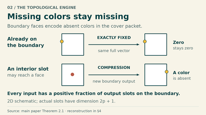
On arbitrarily large product powers, the theorem produces at least boundary slots, where is the number of copies. It also fixes the whole vector of every slot already on the boundary. Merely keeping such a slot somewhere on the boundary would be insufficient: different boundary faces encode different missing colors. Exact preservation protects that information during reconstruction.
The positive boundary fraction is a guaranteed lower bound at every point, not a statistical success rate. The main proof pulls the product construction back along actual successive orbit starts. This is how a theorem about product spaces ultimately constrains the original dynamical system.
11. Colored Covers Complete the Missing Lower Bound
Barycentric subdivision colors the nerve’s vertices so that no simplex contains repeated colors. Group the colors into packets and regularize their proportions near zero total mass. This avoids division by zero while producing continuous cube-valued slot maps.
After compression, reconstruction discards sufficiently small packets. In retained packets, an originally absent color remains absent because its boundary vector was fixed exactly. Every output boundary packet has at least one missing color. Consequently the reconstructed point stays in its original simplex while satisfying a smaller uniform carrier-dimension bound.
This saving is measured against the common nerve-dimension bound. It need not represent a fresh dimension drop at every individual point: a boundary input may already have had a missing color. What matters is a uniform count of possible positive vertex coordinates across the reconstructed image.
The paper preserves two unchanged edge blocks to cover the ends of each interval. A continuous join with an unchanged fallback description handles disappearing alignment. Counting the resulting cells places the image in one finite subcomplex of strictly smaller normalized dimension. Its open-star cover still refines the full orbit cover, contradicting .
Thus . Taking the supremum over covers and infimum over comparison bounds yields the lower inequality, without assuming the infimum is attained. Niu’s upper bound completes equality. Infinite mean dimension excludes every finite comparison bound, so the infinite case follows as well.
12. What the Proof Reveals About Zero Mean Dimension
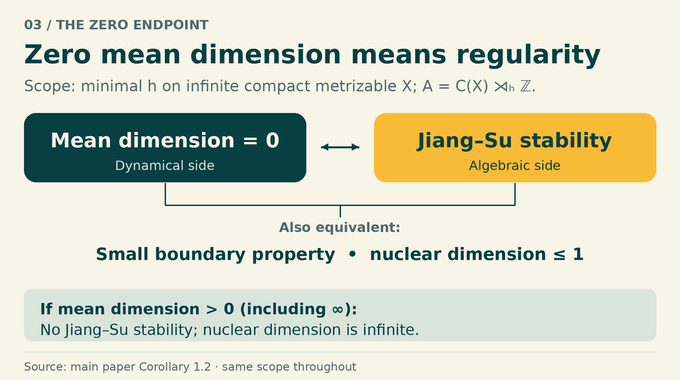
Corollary 1.2 combines the equality with established regularity theorems. Zero mean dimension is equivalent to the small boundary property, Jiang–Su stability and finite nuclear dimension. In this setting finite nuclear dimension actually means .
The small boundary property supplies arbitrarily fine neighborhoods whose boundaries have zero orbit capacity. Jiang–Su stability means , with the Jiang–Su algebra denoted by the calligraphic symbol. Nuclear dimension measures the complexity of finite-dimensional completely positive approximations. For another dimension-related topic, see scalar curvature and Urysohn width.
Elliott and Niu’s zero-mean-dimension theorem supplied stability in the forward direction. The new equality forces the converse through comparison at zero. Positive mean dimension, finite or infinite, therefore implies failure of Jiang–Su stability and infinite nuclear dimension.
The Phillips–Toms conjecture now has an exact integer-action answer: dynamical dimension survives inside the crossed product with a precise one-half scale. The theorem does not settle every amenable-group action. Follow Binary Verse AI for evidence-led explanations that connect each mathematical result to the argument establishing it.
Has the Phillips–Toms conjecture been proved?
Yes, for minimal homeomorphisms of infinite compact metrizable spaces under integer actions. The OpenAI proof establishes the exact equality, including infinite values. It does not establish the conjecture for every possible group action.
Why is radius of comparison exactly half the mean dimension?
The proof connects complex vector-bundle rank to the reduction of real covering dimension. As the rank grows, the construction’s ratio of complex rank to the number of colors approaches one half, yielding the exact constant.
What was missing from earlier proofs?
The sharp upper bound was already known. The challenge was establishing the matching lower bound for arbitrary finite orbit covers without the additional cohomological hypotheses used in earlier lower-bound results.
What role does boundary-preserving compression play?
It forces a positive proportion of cube slots onto their boundaries while preserving every slot vector already on the boundary. This allows the proof to remove colors without losing the information needed to refine the original cover.
Does the proof require the underlying space to be finite-dimensional?
No. The space must be infinite, compact and metrizable, and the homeomorphism minimal. The theorem does not require finite covering dimension.
What happens when mean dimension is zero or infinite?
Zero mean dimension gives radius of comparison zero and, in this setting, nuclear dimension at most one. Infinite mean dimension forces infinite radius of comparison. Positive mean dimension, finite or infinite, implies infinite nuclear dimension.
Why does the proof matter for Jiang–Su stability?
It completes the connection between dynamical complexity and operator-algebraic regularity: for the systems covered, Jiang–Su stability holds exactly when mean dimension is zero.