
A three-layer logic circuit can read every input bit at once and reuse intermediate results freely. OpenAI’s new construction still forces it beyond every constant-times-square-root exponential size bound. The September 23, 2026 paper presents one efficiently computable language whose depth-three Boolean circuits require gates at every sufficiently large input length.
That is the OpenAI Boolean circuit complexity proof’s central claim. It strengthens a specific shallow-circuit lower bound, without resolving P versus NP or demonstrating faster AI software. Released in OpenAI’s October mathematics announcement, it also illustrates why research proofs and benchmark scores are different evidence. Here, the achievement is ruling out every small representation allowed by a precisely defined model.
Table of Contents
1. What OpenAI Proved About Depth-Three Boolean Circuits
Theorem 1.1 of the research manuscript fixes a language , one deterministic Turing machine, and positive integers . That machine decides membership within steps. Let be membership on -bit inputs and the minimum total AND/OR gate count. Then, for every fixed :
The threshold may depend on . The language, machine, and runtime constants cannot. Circuits may change arbitrarily with input length. The bound holds eventually at all lengths, rather than along a convenient infinite subsequence. This rules out changing the language whenever someone asks for a larger lower-bound constant. Choose a million for , and the same evaluator still works. What changes is how far along the input-length sequence the guarantee begins. The theorem supplies no practical crossover length.
1.1. Boolean Circuits: The Key Facts
| Function | One fixed language in deterministic polynomial time |
|---|---|
| Circuit model | Three successive OR–AND–OR layers, read from output to inputs |
| Gate count | All AND/OR gates, including bottom gates and the output |
| Size guarantee | eventually for every fixed |
| Allowed resources | Arbitrary finite fan-in, shared gates, free input negations and constants |
| Unproved stronger claim | A fixed-power exponent , or unrestricted-depth hardness |
2. The Original Boolean Circuit Lower-Bound Problem
Boolean circuit complexity asks how many logic gates are necessary to represent a function. Counting arguments show that most truth tables need enormous circuits. The difficult task is proving such hardness for an explicitly specified, efficiently computable function.
There is no contradiction in putting the language in polynomial time. A Turing machine can carry out many sequential stages. The theorem’s circuit must squeeze its computation into three successive layers. Polynomial-time algorithms have polynomial-size general circuits, but those circuits need not have depth three.
This is a representation bottleneck. Our permanent versus determinant explainer examines another representation problem, in algebraic complexity. Likewise, discrete Fourier transform complexity depends on permitted operations. Neither result transfers automatically between models. Here the central question is whether a shallow classical circuit can reproduce every output exactly, irrespective of how cleverly its gates are wired. Circuit nonuniformity makes that challenge stronger: there is no requirement for a single efficient program to generate the circuit at each length. The lower bound defeats even separately chosen wiring diagrams. The construction is efficient on the algorithm side while allowing this freedom on the circuit side.
3. Why Previous Parity Lower Bounds Stopped at the Square-Root Exponent
Parity returns whether an input contains an odd number of ones. Håstad’s random-restriction and switching method established depth-three circuit lower bounds at the scale. Håstad, Jukna, and Pudlák later improved constants through a top-down approach.
Paturi, Pudlák, and Zane obtained the sharp parity lower bound , matching its upper bound within a constant factor. Thus parity itself cannot exceed every . A larger constant in an existing proof cannot overcome a matching construction.
The new paper therefore changes the hard function. Its qualitative gain is an exponent whose ratio to diverges. As with exponential improvements in Subset Sum, changing an asymptotic rate differs from shaving a polynomial factor. And, as our quadratic sensitivity explainer illustrates, the precise growth comparison determines what a Boolean-function separation actually says.
4. Understanding the OR–AND–OR Circuit Model
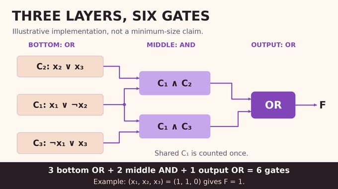
Read the layers from inputs upward. Bottom OR gates form clauses from literals, meaning variables or their negations. Middle AND gates join clauses into conjunctive normal forms, or CNFs. The output OR accepts whenever any middle CNF accepts. These depth 3 circuits allow unrestricted finite fan-in and fan-out, including shared bottom gates. Input negations and constants are free.
For a worked example, define clauses , , and . Use two middle gates for and , then OR their outputs. This implementation has three bottom gates, two middle gates, and one output gate: six total. The shared clause counts once. Input accepts through the first middle gate.
This is an implementation count, not a claim of minimality. Counting only middle gates would be misleading: any Boolean function has a potentially enormous single-CNF representation. Our random 3-SAT guide explains the same clause vocabulary, while quantum circuit lower bounds concern a different gate model.
5. The Central Proof Idea: Low Correlation Forces Large Circuits
Encode the hard function as a sign : positive one on accepted inputs, negative one otherwise. A CNF indicator instead takes values zero and one. The relevant correlation is , with expectation over uniformly random inputs. It measures the imbalance between accepted and rejected points inside the CNF’s satisfying set. This is an unnormalized correlation. A tiny CNF satisfying set automatically has small correlation, even if every point in it is positive. The argument deliberately exploits that fact: an exact middle gate with low correlation must cover only a tiny fraction of the whole cube.
If feeds an exact OR representation, it cannot accept a negative point. Consequently , and small correlation forces , its acceptance density, to be small.
Now imagine covering a substantial positive set with such CNFs. Each covers very little, so many are necessary. This resembles covering a floor with tiny tiles, except overlapping tiles still count against the budget. The proof engineers a slice with positive density and uniformly low CNF correlation, then handles wide clauses separately.
6. Constructing OpenAI’s Polynomial-Time Hard Language
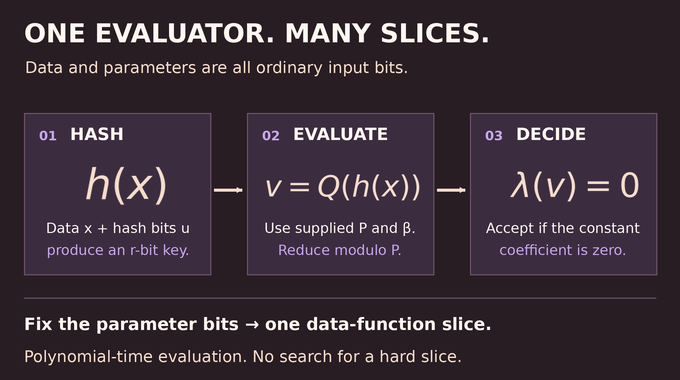
Definition 5.1 starts with data bits, rejects when , and sets . Let be the largest nonnegative even integer satisfying . The input then supplies hash bits, modulus bits, and coefficient blocks of bits each.
The modulus bits encode the monic polynomial over , arithmetic modulo two. Computation occurs in the quotient ring , where polynomials are reduced to degree below .
Hash coordinate defines . Its matrix is Hankel, constant along anti-diagonals, or Toeplitz after reversing data coordinates. With supplied coefficients , acceptance means:
Here extracts the constant coefficient of the reduced representative. Unused bits are ignored. A defensive rejection checks block availability, although the blocks fit whenever .
Monicity makes reduction well-defined even for reducible moduli. Direct hashing and Horner evaluation use bit-array operations, with polynomial Turing-machine overhead. The evaluator neither tests irreducibility nor searches for hard parameters. Fixing those supplied parameters selects a data function called a slice. As a toy illustration of quotient arithmetic, reducing modulo replaces with , since addition and subtraction coincide modulo two. The actual construction uses much larger degrees. The example simply shows why multiplication can return to a fixed-length coefficient array.
7. Random Restrictions and OpenAI’s Signed CNF Restriction Lemma
A random restriction leaves each data variable live with probability , independently, and fixes all others to independent uniform bits. Ordinary simplification need not make every clause narrow when a CNF contains arbitrarily many clauses.
Lemma 3.1 instead represents a restricted width- CNF as a finite signed combination of width- CNFs. Signed means coefficients may be negative, not that logical gates acquire negative inputs. Its controlling parameter is:
The expected total absolute coefficient mass is bounded by . With bounded and , choosing a sufficiently large constant makes this at most two, independently of clause count. Width counts distinct variables in an individual normalized clause. For example, fixing in leaves a two-variable clause. Fixing makes that clause true, so it disappears from the conjunction. The signed expansion addresses clauses that remain too wide after this elementary simplification.
The expansion follows paths of successive clause violations. Counting backwards pairs each possible violated-clause choice with a reciprocal violation count, cancelling dependence on how many clauses are eligible. Classical switching-lemma estimates also avoid a clause-count parameter, but change the normal form. Here the tests remain CNFs. That is the useful distinction in this random-restrictions argument, not a claim that earlier methods ignored formula size.
8. Sunflower Sparsification and Disjoint CNF Partitions
Narrow CNFs still form too large a test family. Lemma 4.1 makes them sparse: for fixed width and any , a CNF on variables partitions into at most CNF indicators. Each retains width at most and has at most clauses, where depends only on .
A sunflower is a family of sets sharing a core, with pairwise disjoint petals outside it. Applied to clauses, branching separates assignments satisfying the core from assignments falsifying it and satisfying the petals. Explicitly requiring the core to be false on the second branch keeps the pieces disjoint.
The proof tracks clause-insertion budgets and bounds branch histories through binary entropy. This controls both leaf count and clause count. Disjointness makes the original indicator exactly the sum of its pieces, avoiding inclusion–exclusion. These are exact identities between indicators, not approximations of satisfying sets. The later error terms come from exceptional restrictions and deleted wide clauses. Keeping these sources separate makes the final probability budget easier to audit. Sparsification also appears in the background of exponential-time hypotheses and SAT, though the present goal is controlling correlation tests. For fixed width, only polynomially many different clauses exist on variables. Limiting each piece to linearly many clauses therefore leaves at most sparse tests. This finite counting bound is what makes a simultaneous probability estimate feasible.
9. How Universal Hashing and Polynomial Interpolation Produce Hard Slices
For the hardness argument, select an irreducible modulus, making a field of elements. A random hash sends each nonzero difference uniformly into that field. On an -dimensional restricted cube, a union bound makes hash-collision probability at most . This uses linear-hash universality, not strong pairwise independence of hash outputs.
When the hash is injective, polynomial interpolation makes evaluations at any distinct cube points independent and uniform. Applying produces unbiased, -wise independent signs. For a fixed sparse indicator , set . Expanding the even moment gives : tuples containing a point just once contribute zero.
Markov’s inequality and a union bound control every sparse test simultaneously. Sparsification with then yields correlation at most for every width- CNF.
Proposition 5.3 chooses , giving mean live dimension . A parameter setting exists whose restriction-failure probability is at most , including dimension tails outside . Averaging proves existence. The evaluator simply reads its parameters, so it need not discover this hard setting. The parameter scales serve separate purposes. Degree , growing like , eventually exceeds the live dimension, which grows like , suppressing collisions. Independence order , growing like , eventually dominates the logarithmic cost of enumerating sparse tests. These comparisons hold with the proof constants fixed.
10. Completing the Proof: From CNF Correlation to the Gate Lower Bound
Fix a proposed exponent constant . Choose , , , and . Next choose constant width large enough for , then take sufficiently large inputs. Combining the restriction lemma with Proposition 5.3 gives, for every width- CNF:
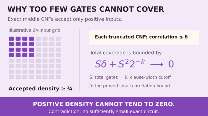
No independence between coefficient mass and good restrictions is assumed. The constant-true CNF also qualifies, so the slice is nearly balanced and eventually accepts at least one quarter of inputs.
Suppose an exact circuit has total gates. Fixing parameter bits cannot increase size. Each of its at most middle CNFs has at most clauses. Deleting clauses wider than enlarges each satisfying set by probability at most , since each deleted clause fails with probability at most . This explains the squared size term: one factor budgets clauses per middle gate, and another budgets middle gates. Sharing bottom gates does not invalidate either upper bound. Counting all gates ensures both budgets remain available even when bottom fan-in is unrestricted.
Correlation bounds the enlarged CNF, with that deletion error added back. Summing across middle gates yields:
Since eventually, the right side is at most , which tends to zero. That contradicts acceptance density of at least one quarter. Arbitrary gives the claimed Boolean circuit lower bounds.
11. What the OpenAI Proof Establishes, What Remains Open, and Lean Verification
The improvement concerns exact depth-three representations with arbitrary bottom width. It establishes neither unrestricted-circuit hardness nor P versus NP. A bound for fixed remains beyond this theorem. Developers should infer no measured SAT, chip-design, or neural-network speedup. As with quantum query complexity, the resource being counted matters.
OpenAI’s published Lean scope covers the fixed polynomial-time language and eventual total-gate bound. The formalization catalogue points to a proof entry combining those results. This article has not rebuilt that Lean development. Formal checking also differs from independent peer review, a distinction explored in our Fermat formalization analysis.
For researchers checking the result, start with the formal theorem’s order of quantifiers and its circuit definition. Then follow the separate evaluator and lower-bound dependencies. Merely finding a theorem statement is insufficient: a comparator challenge can intentionally contain an unproved placeholder, while the implementation proof lives elsewhere. The catalogue distinguishes those roles. For developers, the reusable insight is methodological: fixing parameter bits can expose a hard subfunction without making parameter search part of the computation. That separation is central to why probabilistic existence and a deterministic evaluator coexist here.
The useful lesson for AI readers is to inspect the quantifiers, permitted resources, and verification scope together. For Boolean circuits, the square-root constant barrier is precisely the advance to understand. Keep reading Binary Verse AI for research explainers that connect the theorem to its proof and preserve the limits of what it establishes.
What did OpenAI prove about Boolean circuits?
OpenAI constructed a single polynomial-time decidable language whose membership functions require more than total gates in exact depth-three OR–AND–OR circuits, for every fixed positive constant and all sufficiently large input lengths. The language and evaluator are fixed before is chosen.
Why couldn’t previous parity proofs achieve this result?
Parity has depth-three circuit complexity at the scale, with sharp lower and upper bounds matching within a constant factor. Improving constants cannot exceed every constant multiple of in the exponent, so a different hard function is needed.
How does OpenAI’s proof use random restrictions differently from Håstad’s switching lemma?
The new lemma represents restricted CNFs as signed combinations of narrower CNFs, bounding expected total absolute coefficient mass independently of clause count. Classical switching estimates also avoid a clause-count parameter, but change the normal form. The new tests remain CNFs.
Why is the constructed function polynomial-time computable if its circuits require so many gates?
The lower bound restricts the circuit to three successive layers. A polynomial-time Turing machine can perform a more general sequence of operations. The fixed evaluator therefore computes the language efficiently even though small circuits in the specified shallow model cannot represent it exactly.
Does the proof establish a lower bound of ?
No. It proves , exceeding for every fixed positive constant . It does not establish the stronger bound with any fixed positive .
Does OpenAI’s Boolean circuit proof solve P versus NP?
No. It gives lower bounds for exact depth-three OR–AND–OR circuits. It does not establish comparable lower bounds for unrestricted Boolean circuits or separate P from NP. The constructed language is itself in P.
Has OpenAI’s Boolean circuit proof been formally verified in Lean?
OpenAI published a Lean formalization whose documented scope covers the fixed polynomial-time language, its evaluator, and the eventual total-gate lower bound. The catalogue points to a proof entry combining those results. This article has not rebuilt the Lean development, and formal verification should not be confused with independent peer review.