

A greedy pairing can stop after one edge even when two fit. Finding the best pairing is easy to describe, yet odd cycles have made fast, exact solutions surprisingly difficult. OpenAI’s September 24, 2026 manuscript presents a maximum cardinality matching algorithm running in almost-linear time in the graph’s explicit input size, including the cost of printing its answer.
The claimed improvement removes the classical square-root overhead for sparse general graphs. It uses randomized search, exact matching certificates, and tightly controlled repairs. This is an asymptotic research result, with no reported production benchmark. The interesting advance is how the proof makes global correctness compatible with local work.
Table of Contents
1. What Is Maximum Cardinality Matching, and What Does the OpenAI Proof Establish?
A matching is a set of edges sharing no endpoints. Its cardinality counts edges, and denotes the largest possible count. A perfect matching covers every vertex. A maximal matching merely cannot accept another edge without a conflict.
On the path A–B–C–D, choosing B–C gives a maximal matching of size one. Choosing A–B and C–D gives a maximum, perfect matching of size two. The maximum cardinality matching problem asks for that global optimum.
For a simple, undirected, unweighted graph with vertices and edges, Theorem 1.1 in the manuscript gives:
The exponent correction tends to zero as input size grows. “Almost linear” therefore allows a subpolynomial overhead, not necessarily just logarithms. The computational model charges random bits, finite-word arithmetic, initialization, and output.
| Feature | Verified Scope |
|---|---|
| Input | Simple, undirected, unweighted graph; isolates allowed. |
| Output | Explicit edge list attaining on success. |
| Probability | Success at least for every input. |
| Runtime | Almost linear in , on every computation path. |
| Evidence | Released preprint; practical speedups unbenchmarked. |
2. Why Did the Square-Root Maximum Matching Barrier Persist?
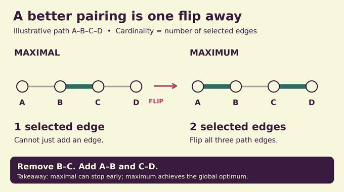
Berge’s criterion says a matching is maximum exactly when no augmenting path exists. Such a path alternates between unselected and selected edges, with unmatched endpoints. Flipping membership adds one edge. On our four-vertex path, flipping all three edges replaces B–C with the two outer edges.
Odd cycles disrupt straightforward alternating searches. Edmonds’ blossom algorithm contracts suitable odd structures, searches the compressed graph, and later expands them. Vertex constraints alone miss the obstruction: assigning one-half to every triangle edge satisfies each vertex’s fractional capacity but totals one-and-a-half edges, while an integral matching has at most one.
The Micali–Vazirani bound is , or including input processing. “Blossom algorithm time complexity” names no single universal implementation bound. Dense graphs also have algebraic approaches at the matrix-multiplication scale.
Bipartite matching already benefits from almost-linear exact integral-flow algorithms. Their row-to-column structure excludes odd cycles. General graphs need additional machinery to control odd blocks. As with other algorithmic barrier results, the input model and output requirement define the advance.
3. How Does the Proof Reduce Maximum Matching to Degree-Three Perfect Matching?
First ask whether a matching of size exists. It leaves vertices unmatched. Connecting every original vertex to new vertices would turn the question into perfect matching, but could create quadratically many edges.
The manuscript replaces those complete connections with a permutation-routing network. Any chosen set of unmatched vertices can reach mandatory sinks through disjoint routes. Splitting each network position into two vertices lets unused positions match internally. The resulting instance has size .
Next replace a degree- vertex by a path containing vertices, attaching old edges at odd positions. Its even positions must match internally, leaving exactly one odd position for an external edge. This enforces the original perfect-matching constraint while limiting degree to three.
Original edge identifiers survive both transformations. A successful perfect matching decodes into actual input edges. This witness requirement separates the theorem from merely estimating an optimum, a distinction also central to our Subset Sum analysis.
4. Factor-Critical Bins and Rows: The New Matching Representation
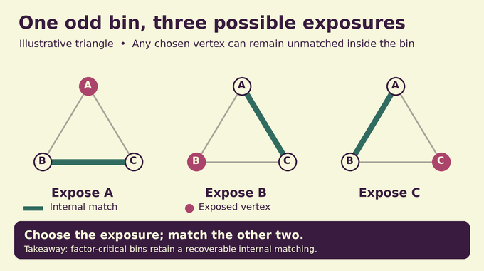
The core procedure stores odd vertex blocks called bins. Each bin is constructively factor-critical: prescribe any vertex to remain exposed, and its other vertices can be matched internally. “Constructively” means the representation retains enough information to recover those edges.
Outside singleton vertices called rows are assigned injectively to bins along original edges. An assigned bin exposes the contact vertex and matches it to its row. A free bin contributes one unmatched vertex. Other vertices sit in explicit matched pairs, while repairs can temporarily set unmatched vertices aside as blockers.
For a triangle, exposing A leaves the B–C edge, while exposing B leaves A–C. Exposure can change without immediately unpacking every nested structure. Stored contraction witnesses support eventual reconstruction.
This postponement needs accounting. Dissolving a contraction tree visits each child once and charges its stored records to the block’s size. Without that bound, a compact representation could conceal repeated expensive expansions. These are matching structures, distinct from the spanning-cycle objective in Barnette’s conjecture.
5. The Hall-Surplus Invariant: Why Multiple Ledgers Matter
Each row distributes units among neighboring bins. Every bin has nominal capacity , so its residual equals capacity minus allocated load. Bin has weight , reflecting its physical size.
Several ledgers maintain different residual floors. Nonnegative debt permits temporary shortfalls. The top ledger supports smooth optimization, intermediate ledgers fund repairs, and the bottom ledger must have zero debt at settled states.
For a bin set , let contain rows whose every neighbor lies inside , and define . These captive rows must spend all their allocation inside the set. Consequently:
Here sums bottom-ledger residuals, and sums bin weights. The first inequality follows from captive-row spending. The second follows from the debt-free residual floor. Since is integral, every nonempty set has surplus at least one.
Consider two bins sharing one captive row. Their deficiency is one. They can accommodate that row while leaving either bin free, but cannot leave both free simultaneously. The invariant supports reassignment without falsely promising unlimited freedom. Adjacent ledger floors differ by one, creating the repair margin used next.
6. How Gains, Blossom Contractions, and Expansions Produce Progress
When an edge joins two bins, try to rearrange row assignments so both become free. Their exposed endpoints can then match across that edge, increasing cardinality by one. That is a gain.
If both cannot be freed, the procedure contracts the relevant minimal tight set with , together with its captive rows. The resulting odd block retains a factor-critical witness. Contraction changes representation, not matching size.
Our two singleton bins plus their captive row illustrate this exactly. If the bins also share an edge, the three vertices form a triangle. One existing row assignment gives one matched edge. Contracting all three preserves that count while allowing any vertex to become the exposure.
Expansion follows an existing bin’s contact to an explicit matched pair. It recruits the contacted vertex as a row and turns its mate into a singleton bin, preserving their edge as the assignment. Slack pays for the edit. If no structural action applies, priced optimization must supply progress on a perfectly matchable instance, subject to failure handling.
7. Local Exact Flow Projection: How the Proof Avoids Global Repairs
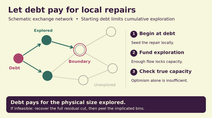
A structural edit can damage residual floors. Recomputing every allocation after every edit would lose the speedup. Instead, projection solves an exchange-flow problem locally, using the starting debt as its work budget.
Exploration begins at bins whose debt is substantial relative to weight. Unexplored boundary bins temporarily receive optimistic sink capacities. This local network upper-bounds what the full exchange network can achieve. Replacing boundary capacities with their true spare capacity supplies a lower bound.
A boundary is explored only when enough flow arrives. Exploration then installs a permanent lower lock proportional to that bin’s spare capacity. Because spare capacity exceeds half its weight at an unexplored boundary, each lock charges newly visited physical size to actual flow. Available flow is bounded by starting debt, limiting cumulative exploration.
If the requested floor is infeasible, the algorithm recovers the full residual source-reachable cut and peels the implicated bins. The one-unit gap between adjacent ledger floors makes removed weight decrease debt in preserved coarser ledgers. Peeling preserves matching size, although free exposures become blockers.
This is a concrete amortization argument: debt pays for both visiting vertices and removing blocks. Exact max-flow information and residual cuts remain necessary despite the optimistic exploration boundary.
The threshold tests bracket an integer flow value. A successful optimistic exploration alone is insufficient: its flow must respect true boundary capacities. Conversely, failure must reveal the complete relevant residual cut, rather than whichever vertices happened to be visited first. Recovering that cut is part of the local projection lemma, not free postprocessing.
8. Priced Logarithmic Steps: How Approximate Optimization Preserves Exactness
The top objective rewards positive allocations and positive slack:
Here is the row–bin incidence set, the bins, and the slack above the top residual floor after debt. A logarithm becomes steep near zero, discouraging the optimizer from exhausting a coordinate.
The pricing engine searches for a circulation direction whose objective gain is large relative to its weighted length. Approximate minimum-ratio circulation machinery supplies that direction. Accepted increments are exact dyadic steps, rational values with power-of-two denominators, preserving the required conservation equations exactly.
Local flow tests use related logarithmic objectives with tiny padded bounds. Their exactness bridge is Lemma 2.2: an exactly conserved real flow whose total violation of integral lower and upper bounds is below one certifies that an integral feasible circulation exists.
Why? Any violated cut inequality would have an integer discrepancy of at least one. Exact conservation bounds that discrepancy by the total violation, contradicting its being below one. Importantly, this certifies feasibility, not that independently rounding each edge works. The accounting includes the return arc too.
Unlike edit distance approximation, approximation here describes an internal optimization tool. The requested matching remains exact.
9. Routing Sparsifiers and Dynamic Forests: The Engine Behind Almost-Linear Time
A useful direction can follow a long graph path. Explicitly traversing every edge after every small step would overwhelm the bound. The backend represents directions through individual edges and paths in maintained forests.
A static routing sparsifier supplies short representative walks while controlling resource loads, including repeated traversals in either direction. During update intervals, frozen forest decompositions express circulations as local correction cycles plus a circulation in a smaller graph. Recursive representations reduce the remaining search cost.
Compression must preserve history. Stable mapped edge copies retain accumulated values when their role changes. Before a copy disappears, its history transfers to persistent storage. Otherwise reorganizing a forest could silently erase an earlier update.
Signed change and absolute motion need separate counters. Traversing an edge forward by five units and backward by five gives zero net change but ten units of motion. The latter pays for refreshes and repricing, preventing cancellation from hiding expensive activity.
That bookkeeping proves the compressed engine is affordable. It is not a claim about general-purpose matrix acceleration or the representation lower bounds discussed in our permanent-versus-determinant explainer.
10. Completing the Proof: From Subcubic Matching to One Uniform Algorithm
For sufficiently large fixed parameter , the subcubic procedure obtains:
Here bounds auxiliary size, and the last term tends to zero with size while stays fixed. The coefficient in is absolute. Phases target a fraction of the remaining deficit, giving logarithmically many phases for fixed parameters, with explicit materialization charged at their boundaries.
Threshold search recovers maximum cardinality because deleting edges makes exact-size feasibility monotone. Accepted answers carry checked witnesses. Randomized failure can yield a false negative, potentially leaving a smaller matching. Error allowances cover adaptive thresholds and internal calls.
A separate fast algorithm for each exponent slack would not establish one uniform program. Section 9 interleaves parameter branches with a deterministic polynomial-time fallback. Each receives weighted instruction quotas, including interruptible arithmetic, allocation, and data movement. The fallback guarantees eventual termination.
For every fixed positive exponent slack, some fixed branch eventually meets it. Weighted scheduling adds only a branch-dependent factor. Summable branch error budgets keep overall failure below one-third without conditioning on which branch finishes first.
A phase’s deficit is the number of additional edges needed for perfection. If the current matching has twenty edges on fifty vertices, that deficit is five. Gains reduce it; contractions and expansions preserve it. This distinction prevents representational activity from being mistaken for actual optimization progress.
The result is classical word-RAM runtime, unlike the input-access measure in quantum query complexity. Charging these implementation details makes the every-path guarantee substantive.
11. What Else Does the Proof Establish, and What Are Its Limits?
| Case | Manuscript Guarantee |
|---|---|
| Sparse: | time. |
| Dense: | time. |
| Prescribed degrees | Find an -factor or decide absence, with bounded randomized error. |
| Weighted optimization | Outside the main theorem. |
An -factor selects edges giving each vertex its prescribed degree . Incidence ports and local permutation networks reduce it to perfect matching with logarithmic expansion. Prescribing degree two gives a spanning collection of cycles, without guaranteeing one connected Hamiltonian cycle.
Finding one matching also differs from counting constrained solutions. Faster construction does not automatically count all matchings or optimize edge weights. Developers still need implementations, crossover measurements, and application-specific validation before expecting deployment gains.
As checked on October 20, 2026, OpenAI’s manuscript catalogue lists this as family 120 without a linked Lean formalization. Its release announcement describes formalizations for many results, not every manuscript. This article explains the submitted argument, rather than claiming independent verification of its entire proof.
The maximum cardinality matching result’s lasting interest is the mechanism: exact combinatorial structure, local debt-funded repair, and compressed optimization working together. Follow Binary Verse AI for research explainers that trace the proof, check its scope, and distinguish a theoretical advance from demonstrated software performance.
What does maximum cardinality matching mean in graph theory?
Maximum cardinality matching is the largest possible set of edges in which no two edges share a vertex. The objective maximizes the number of selected edges, rather than their weights. A maximum matching need not cover every vertex.
What is the difference between maximal and maximum matching?
A maximal matching cannot be extended by adding another edge without a conflict, but it may be smaller than the optimum. A maximum matching contains as many edges as any matching in the graph. Every maximum matching is maximal, but the reverse need not hold.
How do augmenting paths help prove that a matching is maximum?
Berge’s theorem states that a matching is maximum exactly when no augmenting path exists. An augmenting path alternates between unmatched and matched edges and has unmatched endpoints. Flipping its edge membership increases matching cardinality by one.
Why is maximum matching harder in general graphs than in bipartite graphs?
General graphs can contain odd cycles, which complicate alternating-path searches and require additional matching constraints. Edmonds’ blossom algorithm handles these structures through contraction and expansion. The new manuscript develops factor-critical blocks and local repair invariants to control them efficiently.
What is the time complexity of the OpenAI maximum matching proof?
The manuscript states word-RAM time for graphs with vertices and edges, on every computation path. For sparse graphs with , this becomes , improving asymptotically on the classical bound.
Is the new maximum matching algorithm exact or approximate?
It is randomized and returns an explicit exact maximum-cardinality matching with probability at least for every input. The running-time bound holds on every computation path. It is not an approximate-matching guarantee, although an unsuccessful run can fail to return the optimum.
Does the proof also solve weighted matching or guarantee faster practical implementations?
No. Its primary theorem concerns unweighted maximum-cardinality matching, not maximum-weight matching. The manuscript also gives a prescribed-degree -factor result, but reports no production benchmarks demonstrating faster practical implementations.