
Can the shape of an abstract group’s boundary reveal the three-dimensional geometry hidden inside it?
That question has driven research into Cannon Conjecture, one of geometric group theory’s most important longstanding problems. It asks whether every word-hyperbolic group whose boundary at infinity resembles a two-dimensional sphere must admit a geometric action on hyperbolic three-space.
On October 6, 2026, OpenAI released a research manuscript claiming a complete positive solution.
Titled A Modulus Proof of Cannon’s Conjecture, the 31-page paper, dated September 23, 2026, presents a detailed argument based on combinatorial modulus, boundary geometry, continuous limiting functions, and two contradiction methods.
An accompanying Lean formalization provides a machine-checkable version of the claimed theorem.
The proposed breakthrough is specific: OpenAI claims to establish the uniform boundary-modulus bound that earlier mathematical approaches could not prove in full generality.
Understanding that missing step is the key to understanding the paper.
Table of Contents
1. Cannon Conjecture Explained: The Original Mathematical Problem
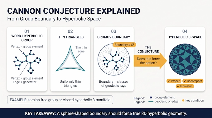
Cannon’s Conjecture concerns word-hyperbolic groups, algebraic structures that exhibit the large-scale geometric characteristics of negatively curved spaces.
A finitely generated group can be represented through a Cayley graph. Its vertices represent group elements, while edges represent multiplication by chosen generators.
A group is word-hyperbolic when geodesic triangles in its Cayley graph are uniformly thin.
Its Gromov boundary records equivalence classes of geodesic rays extending indefinitely outward.
The conjecture asks whether a group whose boundary is topologically a two-sphere necessarily acts geometrically on three-dimensional hyperbolic space.
Cannon Conjecture: Key Mathematical Elements Explained
| Key Element | Mathematical Meaning |
|---|---|
| Conjecture | Cannon’s Conjecture |
| Field | Geometric group theory |
| Starting object | Word-hyperbolic group G |
| Boundary condition | ∂G ≅ S² |
| Expected geometry | Hyperbolic three-space ℍ³ |
| Required action | Proper, cocompact, and isometric |
| OpenAI’s result | Claimed positive resolution |
| Supporting evidence | Written manuscript and Lean formalization |
The condition (\partial G \cong S^2) means the group’s boundary is homeomorphic to a sphere’s surface.
It does not mean the group itself is a sphere.
The challenge is proving that this topological information, combined with hyperbolicity, forces the group to behave like a discrete symmetry group of (\mathbb H^3).
2. The Geometric Barrier: Why a Spherical Boundary Wasn’t Enough
Hyperbolic three-space has a two-dimensional sphere as its ideal boundary.
That naturally suggests the reverse question: if an abstract hyperbolic group has such a boundary, must it come from hyperbolic three-dimensional geometry?
The difficulty is that topology alone does not control distances, distortion, or conformal structure.
Two spaces can be topologically identical while possessing very different metric properties.
Cannon Conjecture: Earlier Mathematical Breakthroughs and Remaining Obstacles
| Earlier Mathematical Tool | What It Established | Remaining Obstacle |
|---|---|---|
| Cannon’s combinatorial Riemann mapping theory | Discrete approaches to conformal coordinates | Quantitative control at all scales |
| Cannon–Floyd–Parry criteria | Conditions involving annular curve families | Establishing those conditions generally |
| Bonk–Kleiner uniformization | Conformal parametrizations of suitable metric spheres | Obtaining the required boundary regularity |
| Bourdon–Kleiner modulus criterion | A usable bounded-modulus condition | Proving that bound universally |
| Marković’s surface-subgroup criterion | An alternative route to Kleinian realization | Finding sufficient separating subgroups |
The analytic route is particularly important to OpenAI’s manuscript.
A theorem associated with Bonk–Kleiner and Bourdon–Kleiner establishes that an appropriately self-similar metric sphere can be parametrized by the round sphere when certain combinatorial curve moduli remain uniformly bounded.
OpenAI’s proof adopts this criterion rather than replacing it.
The unresolved task was demonstrating that the necessary modulus bound follows from the spherical-boundary and hyperbolicity assumptions alone.
That is where the new argument concentrates its effort.
3. OpenAI’s Cannon Conjecture Proof: The Main Theorem
Theorem 1.1 of OpenAI’s manuscript asserts that if (G) is hyperbolic and its boundary is homeomorphic to (S^2), then there exists a homomorphism
[
\rho\rightarrow\operatorname{Isom}(\mathbb H^3)
]
such that the resulting action on hyperbolic three-space is proper and cocompact, with finite kernel.
Each requirement matters.
An isometric action preserves hyperbolic distances. Properness controls how group elements interact with compact regions. Cocompactness means a compact region, together with its group translates, covers the entire space.
A finite kernel permits finitely many elements to act trivially.
The theorem also permits orientation-reversing isometries, avoiding an unnecessary orientation-preserving assumption.
For torsion-free (G), the resulting action is free, producing a closed hyperbolic three-manifold with fundamental group (G).
The manuscript’s architecture is straightforward even though its technical execution is intricate:
- Reduce the conjecture to a uniform combinatorial modulus bound.
- Assume that bound fails and construct a limiting scalar function.
- Exclude exponential growth of the modulus.
- Exclude subexponential unbounded growth.
- Apply boundary uniformization and construct the hyperbolic action.
The rest of the proof establishes why the second assumption cannot hold.
4. Boundary Geometry and the Reduction to Combinatorial Modulus
Section 2 builds the geometric foundation needed for the contradiction argument.
The authors equip (Z=\partial G) with a visual metric and examine the action of group elements on that boundary.
Their expansion formula, Lemma 2.1, shows how translating along a sufficiently long geodesic effectively magnifies a small boundary neighborhood.
Importantly, the formula also controls points outside the magnified region.
This two-sided control becomes essential when comparing different expansions later.
Additional lemmas establish packing estimates, doubling behavior, and controlled paths on the boundary.
4.1. The Modulus Quantity (M(n))
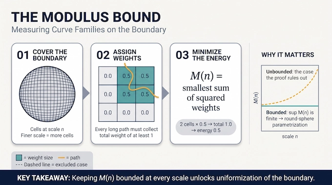
At a fine scale (r_n=a^{-n}), the boundary is covered by cells centered on a separated net.
Each cell receives a nonnegative weight (\omega(q)).
An admissible assignment requires every path of a prescribed minimum diameter to meet cells whose total weight is at least one.
The combinatorial 2-modulus minimizes the squared weight sum:
[
M(n)=\min_{\omega}\sum_{q\in T_n}\omega(q)^2
]
subject to the path-admissibility condition.
Theorem 2.5 reduces the problem to proving
[
\boxed{\sup_n M(n)<\infty}
]
The bound means that the combinatorial energy required to control these macroscopic curve families cannot grow without limit as the covering becomes finer.
If it holds, existing uniformization theory supplies a quasi-Möbius parametrization of the boundary by the round sphere.
OpenAI’s main technical task is therefore to eliminate every possible way in which (M(n)) could become unbounded.
5. Constructing a Scalar Limit From Unbounded Modulus
Section 3 begins with the opposite assumption:
[
\sup_n M(n)=\infty
]
The authors select record scales at which the modulus becomes increasingly large, retaining inequalities that compare different resolutions.
The first major step is crossing duality.
Inside a coordinate rectangle, horizontal and vertical curve crossings constrain each other. Using a finite-dimensional extremal-length argument, Lemma 3.3 constructs transverse admissible weights with squared energy bounded by a constant multiple of (1/M(N)).
As (M(N)) grows, that energy approaches zero.
5.1. From Discrete Weights to Continuous Functions
The authors turn these weights into functions describing the cost of moving across the rectangle.
A careful regularization using two path envelopes produces continuous functions (H_N).
Their level sets contain connected separating continua. A path whose endpoint values straddle a given level must intersect the corresponding continuum.
This construction preserves small local oscillation energy while introducing the continuity needed for later comparisons.
Annular estimates then control variation across neighborhoods of different sizes.
Proposition 3.7 extracts a locally uniformly convergent subsequence:
[
H_N\longrightarrow u
]
Here (u) is continuous, nonconstant, and takes values between zero and one.
A finite measure (\mu) also emerges, satisfying an estimate of the form
[
(\operatorname{osc}_{B(x,s)}u)^2
\le C\mu(B(x,Cs))
]
This inequality connects changes in the limiting function to measurable mass.
Another key ingredient, Lemma 3.8, compares two functions along common separating level sets.
Together, these results create the analytical machinery needed to contradict unbounded modulus growth.
6. The Exponential-Growth Contradiction
Section 4 considers the first possibility: the record modulus grows at an exponential rate.
Under this assumption, Proposition 3.7 gives additional regularity. The limiting function (u) becomes locally Hölder continuous.
That matters because Hölder continuity provides quantitative control over how the function changes at small scales.
6.1. Magnifying Nonconstant Variation
Lemma 4.1 selects regions where (u) genuinely varies and magnifies them through carefully chosen group transformations.
After normalization, the transformed functions converge to a nonconstant limit on a punctured sphere.
The puncture corresponds to the point excluded by the limiting expansion.
The manuscript then compares this limit with its transforms under other group elements.
Lemma 4.3 establishes a restrictive relationship: when two transformations have distinct punctures, one transformed function must be constant across the non-locally-constant region of the other, apart from the stated exceptional point.
This follows from the separating continua and the vanishing oscillation-energy comparison.
6.2. Why a Second Magnification Produces a Contradiction
The authors magnify the limiting function again.
They first control possible repeated punctures using information about stabilizers of boundary points.
The second magnification produces two regions with separated function-value ranges, while each region contains genuine variation.
Applying the transform-comparison lemma forces one transformed function to take the same value in both regions.
But their value ranges are disjoint.
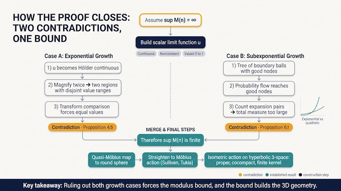
That contradiction establishes Proposition 4.5: exponential unbounded modulus growth is impossible under the hypotheses.
The proof has excluded its first escape route.
7. Subexponential Growth: The Probability-Flow Construction
An unbounded sequence can grow more slowly than every exponential rate.
Section 5 handles this remaining possibility using a different strategy.
The authors construct a tree of small boundary balls. Each node records a center, a geometric scale, and an interval of values attained by (u).
Children occupy smaller scales and carry nested value intervals.
Some nodes are designated good because they exhibit two spatially separated regions with sufficiently separated function-value ranges.
The objective is to prove that substantial probability repeatedly reaches such nodes.
7.1. Transition Probabilities and Capacity
Each parent distributes probability among separated children.
The transition probabilities satisfy two types of estimates.
Linear bounds control the probability accumulated along branches. Quadratic bounds relate probabilities to squared lengths of value intervals.
Those squared lengths can then be compared with the finite measure obtained in Section 3.
Lemma 5.1 establishes that a node failing the good-node condition has many separated children carrying substantial portions of its value interval.
Lemma 5.2 supplies a capacity estimate that guarantees suitable transitions even when intervals become very small.
The authors then distinguish good and non-good nodes through their different quadratic probability bounds.
The resulting flow forces a definite amount of probability onto good nodes at arbitrarily deep generations.
This is the purpose of the construction: it turns persistent function variation into many separated geometric configurations that can be compared simultaneously.
8. Comparing Expansions: The Final Counting Contradiction
Section 6 converts the good-node configurations into a contradiction involving the finite measure (\mu).
The authors choose a large generation containing substantial good-node probability.
After grouping nodes by their geometric patterns and comparable probability sizes, they obtain a large family of expansions.
Each expansion carries two separated target regions where the transformed function exhibits controlled variation.
The analysis then considers pairs of expansions whose punctures are sufficiently far apart.
8.1. The Pair Alternative
Lemma 6.4 proves that each sufficiently separated pair must have an endpoint at which the corresponding transformed function exhibits a definite oscillation.
The proof again uses the scalar functions and separating continua from Section 3.
If neither endpoint had sufficient variation, the finite-cell level-comparison lemma would produce a contradiction with the vanishing oscillation energies.
Thus every eligible pair creates a measurable cost.
The oscillation-measure estimate converts that cost into a lower bound on the measure of a small source neighborhood.
8.2. Why the Total Cost Becomes Impossible
The final step counts how often these neighborhoods can overlap.
The boundary expansion formula controls their images, while packing estimates and separation between source centers limit their multiplicity.
A large collection of eligible pairs therefore forces substantial total measure.
But the total available measure remains finite.
The paper’s estimates ultimately produce an inequality of the form
[
a^{\gamma Dn}\le C(k_0+Dn)^2
]
with (a>1) and fixed positive constants.
The left side grows exponentially in (n). The right side grows only quadratically.
They cannot satisfy this inequality for arbitrarily large (n).
Proposition 6.1 therefore excludes unbounded subexponential growth.
Both routes to unbounded modulus have now been eliminated.
9. Completing the Proof: From the Boundary to Hyperbolic Three-Space
Section 7 combines the two contradictions.
If (M(n)) were unbounded, the record-selection argument would lead either to exponential records or to the subexponential case.
Proposition 4.5 excludes the former. Proposition 6.1 excludes the latter.
Consequently,
[
\sup_n M(n)<\infty
]
Theorem 2.5 then provides a quasi-Möbius homeomorphism between the visual boundary and the round sphere.
But uniformizing the boundary is not quite the final conclusion.
Proposition 2.6 supplies the remaining bridge.
The group action becomes uniformly quasiconformal after boundary conjugation. Using the invariant-conformal-structure method associated with Sullivan and the circumcenter construction developed by Tukia, the authors straighten it into a Möbius or anti-Möbius action.
These transformations extend to isometries of hyperbolic three-space.
Finally, the paper uses the group action on ordered triples of distinct boundary points to establish properness and cocompactness.
The kernel is finite.
This completes the proposed proof of Theorem 1.1.
10. What the Result Establishes for Hyperbolic Groups
Section 8 derives two principal consequences.
Corollary 8.1 states that a torsion-free hyperbolic group with spherical boundary is the fundamental group of a closed hyperbolic three-manifold.
The manifold need not be orientable.
Corollary 8.2 derives further structure using established three-manifold and group-theoretic theorems.
Some finite-index subgroup has the form
[
\pi_1(\Sigma)\rtimes\mathbb Z
]
where (\Sigma) is a closed connected orientable surface.
In geometric terms, this corresponds to virtual fibering over a circle.
The paper also derives positive virtual first Betti number, virtual compact specialness, and residual finiteness for the torsion-free groups covered by the corollary.
These are substantive mathematical consequences, not separate claims that OpenAI independently reproves the earlier underlying theorems.
The new contribution is the claimed geometric realization that makes those established results applicable.
11. Cannon Conjecture Lean Proof: What the Formalization Establishes
Alongside the manuscript, OpenAI published a Lean implementation containing the theorem OAI.CannonRelease.cannon.
Its statement begins with a group equipped with Cayley-graph data, a uniformly thin-triangle hypothesis, and a boundary homeomorphism with (S^2).
Its conclusion provides an isometric action on (\mathbb H^3) satisfying properness, cocompactness, and finite-kernel conditions.
The main theorem invokes supporting formalized results for boundary uniformization and the construction of the geometric action.
OpenAI also supplies scope documentation and a comparator configuration identifying the solution module, theorem name, and permitted axioms.
These materials allow the formal statement and its dependencies to be inspected.
The comparator’s separate challenge template contains a sorry placeholder, but the published solution module provides a theorem proof rather than using that placeholder as its conclusion.
A formal proof is intended to let Lean check every justified inference within the specified formal system.
The important remaining distinction is between a publicly available formalization and an independently reproduced audit of its full dependencies, assumptions, and correspondence to the paper.
As of October 11, 2026, OpenAI’s published manuscript and Lean files provide concrete evidence for the claimed resolution, but this article does not treat independent expert acceptance as established.
12. Why OpenAI’s Cannon Conjecture Proof Matters
The mathematical significance of this result lies in the connection it claims to make unavoidable.
A word-hyperbolic group with a spherical boundary would not merely resemble a three-dimensional hyperbolic object from far away. It would admit an actual geometric realization in hyperbolic three-space.
OpenAI’s proposed proof reaches that conclusion through a carefully structured sequence: boundary expansions, combinatorial modulus, scalar limiting functions, exponential-growth rigidity, probability flow, and a final measure-counting contradiction.
Its strongest feature is how these components address the precise quantitative barrier left by earlier uniformization methods.
If the argument and formalization withstand full scrutiny, Cannon Conjecture becomes a theorem connecting boundary topology to three-dimensional hyperbolic geometry in remarkable generality.
For a closer examination, read the original 31-page paper and its Lean formalization side by side. Sections 3 through 6 contain the core new mathematical work.
Follow Binary Verse AI for detailed, research-grounded explanations of AI-generated mathematical proofs, their technical mechanisms, and the results they establish.
1. What is Cannon’s Conjecture in simple terms?
Cannon’s Conjecture asks whether every word-hyperbolic group whose boundary at infinity looks like a two-dimensional sphere must arise from three-dimensional hyperbolic geometry. It connects abstract algebraic structures to geometric spaces. For torsion-free groups, a positive solution means they are fundamental groups of closed hyperbolic three-manifolds.
2. Has OpenAI solved Cannon’s Conjecture?
OpenAI released A Modulus Proof of Cannon’s Conjecture, dated September 23, 2026, claiming a complete positive resolution. The corresponding Lean theorem and implementation are publicly available. However, as of October 11, 2026, I have not established that independent mathematicians have completed and accepted a comprehensive verification of this particular proof.
3. How does OpenAI’s new proof overcome the previous mathematical barrier?
Earlier work provided criteria for recognizing when a group’s spherical boundary has the necessary conformal geometry, but those criteria had not been established in full generality. OpenAI’s manuscript attempts to fill that gap by showing the required combinatorial modulus remains uniformly bounded. It rules out both exponential and subexponential forms of unbounded growth.
4. Does Lean verification guarantee that OpenAI’s Cannon Conjecture proof is correct?
Lean can mechanically check a formal proof relative to its definitions, axioms and trusted logical foundations. OpenAI’s released formalization states a proper, cocompact action on hyperbolic three-space with finite kernel. Independent examination is still important to confirm that every definition and assumption matches the intended mathematical statement and that the entire implementation reproduces successfully.
5. Why is Cannon’s Conjecture important, and how is it related to the Poincaré Conjecture?
Both concern the relationship between topology and three-dimensional geometry, but they answer different questions. The Poincaré Conjecture characterizes certain simply connected three-manifolds. Cannon’s Conjecture instead asks whether the boundary topology of an abstract hyperbolic group forces a hyperbolic three-dimensional realization. A confirmed proof would significantly strengthen this bridge between group theory and geometric topology.