
A wave can conserve positive energy and still grow without bound at one point. OpenAI’s September 2026 preprint proves this kind of nonlinear Schrödinger equation blowup for a scalar defocusing model on the twelve-dimensional torus. For a suitably chosen large odd power, every initial condition in a nonempty open set of a high Sobolev space produces a finite-time singularity. At its center, the wave grows at the exact rate predicted by self-similar scaling. Earlier work already constructed defocusing singularities. Here the result is their persistence under small perturbations in the physical Sobolev norm, with a direct consequence for randomly sampled initial data. Read the original preprint.
In the equation, is complex-valued, is time, is the spatial Laplacian, and is the odd nonlinear power. The domain is periodic with period in each coordinate.
Table of Contents
1. What OpenAI’s Nonlinear Schrödinger Equation Blowup Proof Establishes
Theorem 1.1 fixes a suitable odd power and then a finite integer . It produces a nonempty open set . The Sobolev norm measures closeness of the data and of their spatial derivatives up to the chosen order. The result allows small changes in any direction in this space, including perturbations that break the radial symmetry of the profile used in the proof.
| Feature | Proven Result |
|---|---|
| Equation | Scalar, unforced defocusing NLS on the twelve-dimensional torus |
| Nonlinearity | A selected sufficiently large odd power |
| Initial Data | A nonempty open set in for a fixed finite integer |
| Singularity | Finite time, with a positive rescaled amplitude limit at the center |
| Gaussian Data | Positive blowup probability for every Fourier decay exponent |
Each solution stays continuous in until its own finite time and is continuously time differentiable in on that interval. Its amplitude diverges at a fixed point in physical space. Since embeds into continuous functions here, this forces the norm to diverge and rules out continuous continuation through .
2. The Original Problem of Global Regularity for Defocusing NLS
Both energy terms are nonnegative in the defocusing nonlinear Schrödinger equation. The first measures spatial gradients. The second penalizes large amplitude through a power integral. Mass, the integral of , is also conserved. Together these quantities bound the norm and the norm throughout smooth evolution.
Local existence comes from a different estimate. For in dimension , products of functions stay in . For odd , the nonlinearity is a polynomial in and its complex conjugate, so a fixed-point argument for the time integral equation yields a unique local flow. Iteration requires control of the norm used in that argument. For a related dispersive estimate, see the local smoothing conjecture explainer.
3. The Energy-Supercritical Obstacle for Conservation Laws
On Euclidean space, rescale a solution by replacing its time and space arguments with and , then multiply by , where . The time derivative and Laplacian both contribute two powers of . The prefactor makes the nonlinear term scale by the same amount. In a homogeneous Sobolev norm of order , the derivative contributes and the change in spatial volume contributes . The exponent of the norm is zero at the critical index.
On the fixed torus, the Euclidean calculation describes the scales seen when zooming in near a point. In twelve dimensions, even the illustrative cubic power gives , far above the energy level. To see the gap, take a smooth compactly supported bump and apply the spatial and amplitude scaling above, placing its shrinking support inside one periodic cell. Both energy terms then scale by . The height increases while the energy of these test functions decreases. This is a comparison of snapshots. The later profile construction supplies an actual time evolution.
4. Earlier Defocusing Blowup Proofs and the Stability Question
Tao’s forced system exposed a weakness in arguments based solely on conservation and scaling. Later scalar results removed the forcing, including a periodic construction that allowed nonradial solutions. The remaining issue was the size of the blowup family in the ambient space of initial data. Finite codimension means that finitely many constraints still have to be met. A full Sobolev neighborhood can absorb perturbations in those directions too.
| Research | Setting and Family |
|---|---|
| Tao | A specially designed forced, vector-valued system |
| Merle, Raphaël, Rodnianski, and Szeftel | Radial, scalar type-II blowup on whole space for four dimension–power pairs, in finite-codimension families under the stated profile nondegeneracy condition |
| Cao-Labora, Gómez-Serrano, Shi, and Staffilani | Nonradial periodic blowup for the cubic equation in dimension eight, in a finite-codimension family |
| Buck, Carballeira, Gómez-Serrano, and Shi | Schrödinger-scale blowup from smooth, compactly supported radial data on whole space, in dimension and power pairs , , and , in finite-codimension families |
The earlier hydrodynamic constructions use a spatial scale with . OpenAI’s manuscript combines the Schrödinger scale of Buck and collaborators with openness on a periodic domain. For a separate scalar NLS result, see the Muse Spark blowup explainer.
5. How the Self-Similar Blowup Forms: Scaling, Amplitude and Phase
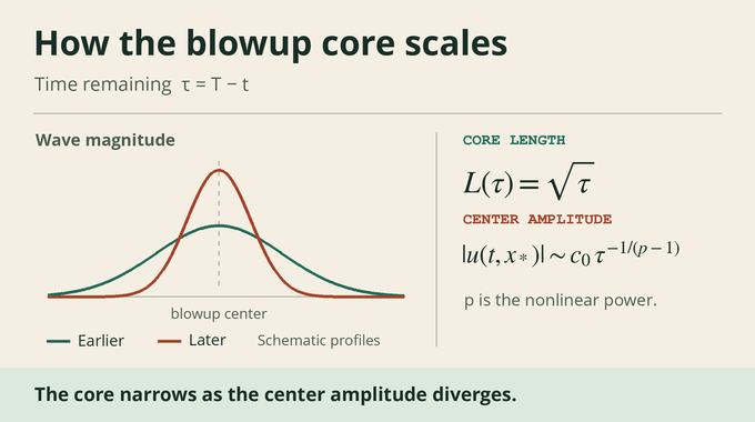
Write for the time remaining. Shrinking distances by the length scale puts the Laplacian on the same scale as the time derivative. Balancing these terms with the nonlinearity gives the amplitude factor , where . The rescaled position keeps the core at a fixed size, and logarithmic time sends the finite endpoint to infinity.
The similarity ansatz takes the following form, with constant phase , real phase frequency , and rescaled wave . The complex power rotates the phase by an angle proportional to the logarithm of the remaining time. Its modulus is one.
In these coordinates, the time derivative of similarity time is the reciprocal of the time remaining, while the derivative of rescaled position is the position divided by twice the time remaining. Substituting and canceling the common power of gives the profile equation below when the rescaled wave is stationary and equals the spatial profile. The gradient term records the drift from the changing spatial scale.
In the torus solution the rescaled wave approaches this profile locally. At the center its modulus approaches the profile’s positive center amplitude. Theorem 1.1 gives the exact pointwise limit
For example, reducing the remaining time to a quarter halves the spatial scale and multiplies the leading center amplitude by . The paper calls this type-I blowup because the shrinking length and growing amplitude follow the equation’s similarity scaling.
6. Constructing the Blowup Profile: From a Pressurized Core to a Free Exterior
Section 3 writes the radial profile as , with positive amplitude and real phase . The nonlinear coefficient plays the role of pressure. Along convergent subsequences as tends to zero, the limiting profile is flat and equal to one inside a core, where the pressure tends weakly to the positive parameter . Outside the core the pressure vanishes in the limit. The exterior is therefore governed by the free similarity equation. The finite-power profile is smooth across the transition. For related elliptic profile analysis in a supercritical setting, see the Lane–Emden conjecture explainer.
The exterior solution is a Tricomi confluent hypergeometric function selected by its slow, nonoscillatory asymptotic form. Its value fixes the normalization at the interface. Its radial derivative must vanish there to match the flat core. The matching residual is complex, which gives two real conditions for two real variables, the phase frequency and the core radius. The certified residual has Brouwer degree minus one on a small parameter disk. This integer is preserved under continuous deformations that keep zeros off the boundary. With the finite-power matching estimates in place, the nonzero degree forces a zero and yields a genuine profile. A different elliptic interface problem appears in the one-phase Bernoulli explainer.
7. The Spectral Stability Proof: Excluding Unwanted Growing Modes
Linearizing about couples a perturbation to its complex conjugate. The analysis tracks both channels after complexification. Radial symmetry lets the authors split the resulting system into spherical harmonics indexed by angular degree . Each mode evolves like in similarity time. Zeros of the limiting determinant encode when solutions regular at the origin match outgoing solutions at infinity.
Laguerre recurrences bound the tails in the special-function expansions. For low angular degrees, exact rational comparisons certify winding counts of the determinants and the profile-matching degree. A complex-path multiplier handles the high angular degrees of the limiting problem. At finite power, a uniform outgoing estimate keeps roots from escaping to arbitrarily large temporal or angular frequencies. Convergence of the constrained pressure problem carries the bounded spectral count across, with algebraic multiplicity.
Theorem 4.1 classifies modes with . There is one phase direction at , twelve translations at , and one blowup-time direction at . These directions change how the singularity is centered, phased, or timed. The classification excludes extra modes in the stated half-plane and generalized modes above the symmetry eigenvectors. The next step turns this spectral information into decay estimates for the evolution.
8. Transferring the Blowup Construction to the Twelve-Dimensional Torus
Rescaling the fixed periodic cell gives a torus whose period grows like . The authors cut off the whole-space profile within that expanding cell, introducing a small error. They also transport the symmetry coordinates to the periodic problem. On each fixed similarity-time interval, a sequence of expanding tori can approximate whole space on bounded regions. Such a limit can miss perturbations whose Sobolev norm is carried far from the core.
Section 5 controls the full scale-dependent Sobolev norm using a dissipation estimate with a local observation term. This decay refers to the norm in similarity variables. The free evolution in those variables already gives decay at the two Sobolev orders used in the estimate. Local convergence passes the observation term to the whole-space limit. The contribution of the full initial norm is still present and decays over the interval, even for sequences whose local limit vanishes. The proof first chooses a long time step and then a sufficiently large initial torus scale. That order makes the stable projection at the end of the step at most one eighth of the initial stable norm. Each new step starts on a larger torus, so the same estimate can be reused.
9. From a Stable Graph to an Open Set of Blowup Initial Data
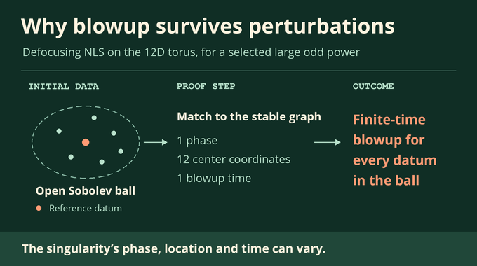
With phase, center, and time held fixed, a perturbation splits into a stable part and fourteen symmetry coordinates. The stable part can be advanced forward by contraction. The symmetry coordinates are chosen from a convergent sum of future errors so that the full perturbation decays. Section 6 packages this choice into a continuous stable graph over the stable directions. It depends on the torus scale, which itself changes when the candidate blowup time changes.
The decisive move takes place in the physical initial-data space. For every datum near a smooth reference wave, the authors vary the phase, twelve center coordinates, and the blowup time. They compare the resulting symmetry coordinates with the graph’s prescribed values. Around the reference datum, the parameter-to-coordinate map has an invertible linear leading part. The remaining errors are uniformly smaller than that linear map on the boundary of a small parameter ball. Brouwer degree then supplies a match for every physical datum sufficiently close to the reference. Continuity of the graph suffices for the argument.
Once matched, the rescaled perturbation decays, and the profile supplies the pointwise singularity. This is stable NLS blowup in the physical sense. One Sobolev ball of input data produces singular solutions with parameters allowed to vary for each solution.
10. Why Gaussian Fourier Initial Data Can Also Blow Up
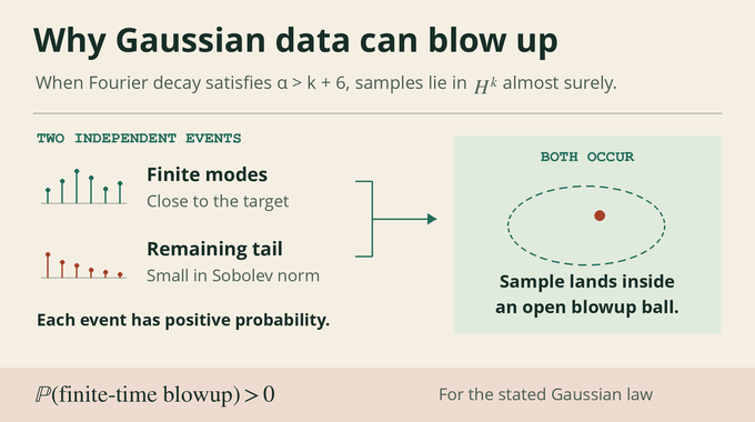
Corollary 1.2 samples independent standard complex Gaussians at frequencies . The Fourier coefficient is , where and controls decay. The expected squared Sobolev norm is proportional to the sum of . Counting frequencies in successive dyadic shells shows that summability requires the weight to decay with an exponent greater than twelve. This gives the paper’s condition . For related Fourier background, see the Fourier series convergence explainer.
Full support follows by approximating any target by finitely many coefficients. The finite Gaussian vector has positive density, so it can land as close as needed to that target segment with positive probability. Independently, its remaining tail has a small expected squared norm and can be small with positive probability. Both events can therefore occur together. Every nonempty ball receives positive probability, including a ball in the open blowup set.
The manuscript frames this as a counterexample to a universal eventual-global-existence assertion motivated by the random-tensor open problem of Deng, Nahmod, and Yue. That assertion would give each energy-supercritical dimension and power a decay threshold beyond which the Gaussian flow is almost surely global at every Sobolev index in a specified interval. Here the index lies in that interval for every admissible decay exponent, and the blowup probability is positive. The probability can depend on the exponent.
11. What the Proof Establishes and Where It Applies
The open-set and Gaussian conclusions concern dimension twelve and an odd power selected sufficiently large, with chosen afterward. OpenAI’s scope note formulates the Lean result for arbitrarily large selected odd powers. The manuscript also gives smooth deterministic examples on higher-dimensional product tori by extending a twelve-dimensional solution constantly in the extra coordinates. The extra Laplacian terms vanish, and blowup occurs along the fiber over the original center. This extension provides existence on those tori. Stability against perturbations depending on the extra coordinates remains outside the argument.
The Lean source states the stable and Gaussian results using its formal definitions. The formalization accompanies OpenAI’s October mathematics release. Matching those definitions to the paper is a separate mathematical review. Appendix A’s Python verifier recomputes finite integer and rational comparisons. The paper’s analytic arguments connect those checks to the profile degree and spectral count. Read the Lean scope note, inspect the theorem declarations, or find the arithmetic verifier.
The significance of this nonlinear Schrödinger equation blowup theorem is the passage from one singular profile to a whole neighborhood of singular evolutions. That neighborhood is what makes blowup visible to a prescribed Gaussian law, even at high regularity. Follow Binary Verse AI for more research explainers on PDE regularity and formal verification in PDE.
Can the defocusing nonlinear Schrödinger equation blow up in finite time?
Yes. The preprint proves stable finite-time blowup for a scalar energy-supercritical defocusing NLS on the twelve-dimensional torus. The theorem applies to a selected sufficiently large odd power and a nonempty open set of initial data.
Why does positive conserved energy fail to prevent blowup?
The conserved energy controls the gradient in and the amplitude in . The scaling-critical Sobolev index exceeds one, so continuation in the regime studied here requires control beyond the energy level.
What does stable self-similar blowup mean?
The solution develops a singularity with a controlled scaling pattern. Blowup persists under sufficiently small perturbations of the initial data in the specified Sobolev norm. The blowup time and location can change.
What is the blowup formula proved in the paper?
At a suitable point , the theorem gives . The center amplitude therefore diverges at rate as the finite blowup time approaches.
Does the proof establish blowup for the three-dimensional Schrödinger equation?
The Sobolev-open theorem applies in twelve dimensions. Earlier work obtained scalar defocusing blowup in three dimensions for power 27, with a finite-codimension family of radial whole-space data.
Does Gaussian initial data blow up with probability one?
The corollary proves a strictly positive probability of finite-time blowup for the specified Gaussian Fourier laws. The probability can depend on the Fourier decay exponent. An assertion of probability-one blowup would require a separate argument.
Has the entire proof been formally verified in Lean?
OpenAI released Lean proofs of formal statements for stable blowup and positive-probability Gaussian blowup. Establishing that the formal definitions capture the intended analytical claims requires a mathematical comparison. The separate Python verifier checks the finite arithmetic used in the profile and spectral arguments.