
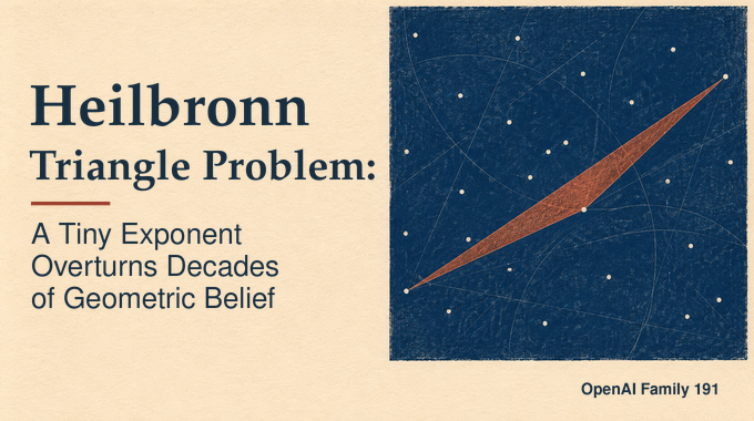
Put four dots at the corners of a unit square. Whichever three you join, the triangle covers half the square. With a million dots, how much area can you guarantee for the skinniest triangle? The Heilbronn triangle problem asks how well the best arrangement can do as the number of dots grows. OpenAI’s September 2026 manuscript proves that, for every sufficiently large point count, some arrangement beats the classical inverse-square scale by a fixed positive power. The paper’s explicit exponent is about . It stays fixed as the point count grows.
Table of Contents
1. What Is the Heilbronn Triangle Problem?
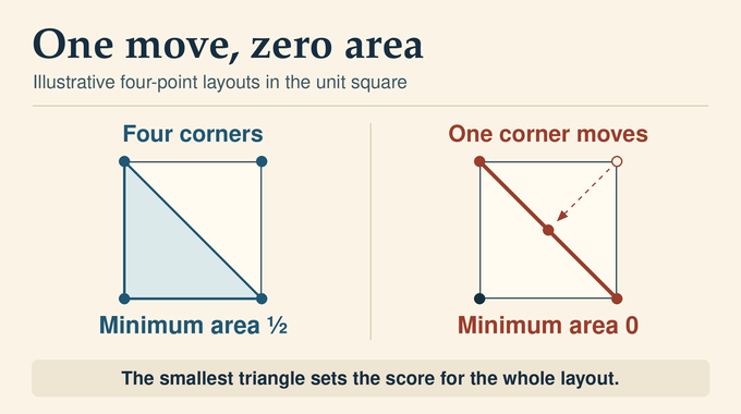
Choose a set of distinct points in the closed unit square. Write for the least area among all triangles with three different vertices in that set. Now allow the points to move and call the largest attainable value . You choose the arrangement. Someone who sees your choice picks the worst triple.
Each triangle in the four-corner example has unit base and height, so the minimum is . Move the top right corner to the centre. The centre lies on the diagonal between the two opposite corners. The minimum drops to zero even though all three points on that diagonal are distinct and well separated.
2. The Heilbronn Conjecture and Four Decades of Limited Progress
Heilbronn conjectured an upper bound of . Erdős showed why that scale looked plausible. For an odd prime , take the points with coordinates and the least nonnegative residue of modulo , with . No line meets the finite-field parabola in three distinct points. Back on the integer grid, twice the area is therefore a nonzero integer. Dividing both coordinates by gives a minimum area of at least for points.
In 1982, Komlós, Pintz and Szemerédi gained a factor of . As in the study of square-difference-free sets, the question became how large a set could avoid a forbidden pattern. They made each small triangle an edge of a hypergraph on the sampled points. Removing short cycles then let them extract a larger independent set, a subset containing no forbidden triple. This disproved the original conjecture. A weaker prediction survived because a logarithm grows more slowly than every fixed positive power.
3. OpenAI’s New Lower Bound: What the Tiny Exponent Changes
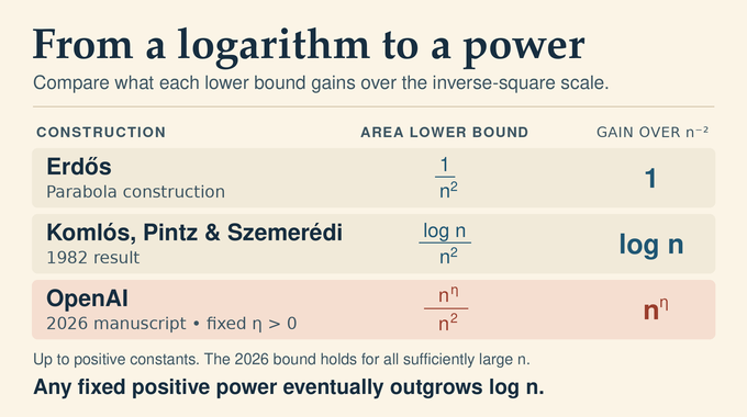
Theorem 1.1 of the manuscript gives absolute constants and an integer such that, for every integer ,
Multiply the guaranteed area by . On this scale Erdős reaches a constant, Komlós and colleagues reach a logarithm, and OpenAI reaches a power. Squaring the point count doubles the logarithm. For the power, the multiplier is itself, which eventually exceeds any fixed number.
The relaxed Heilbronn conjecture allowed a different constant for every and predicted eventually. Choose . The ratio of the new lower bound to that proposed upper bound is , which grows without limit. The conjecture required this instance to hold.
4. Inside OpenAI’s Proof: A Six-Stage Roadmap
OpenAI attributes the results in its October release to an internal frontier model. These stages reconstruct the manuscript’s logic. Their order reflects dependencies between lemmas.
- Projective representation. Give each planar point three integer coordinates. The third acts as a denominator, letting one integer determinant measure the area of a projected triangle.
- Finite-field encoding. Give each column a label. Encode a test for three different labels in the digits of the columns, so a small determinant can occur only when labels repeat.
- Lattice counting. For repeated labels, count the lifts, the integer columns with the prescribed residues, that realize each small nonzero determinant, allowing for unequal spacing in different directions.
- Auxiliary congruence. At determinant zero, whole planes of possibilities survive. A second modulus excludes short relations among distinct residues and controls the remaining planes.
- Random sampling. Combine the two restrictions and sample their integer lifts. A weighted count converts the arithmetic information into a probability for one troublesome triple.
- Deletion and normalization. Start with twice the desired number of columns. Delete the violations, project the survivors and translate the determinant threshold back into area.
5. Turning Triangle Areas Into Integer Determinants
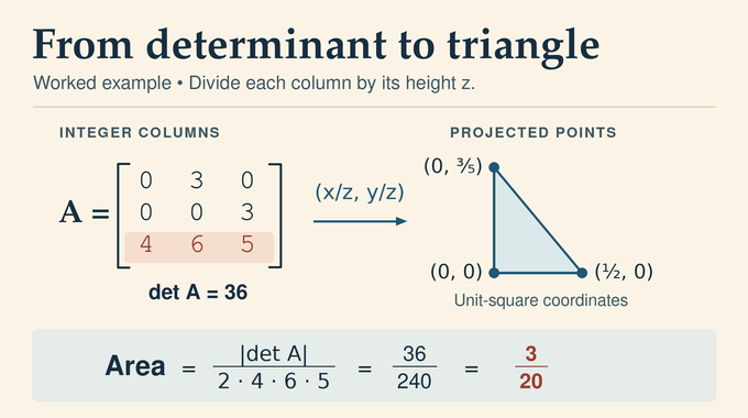
Draw the ray from the origin through the tip of an integer column . It meets the plane of height one at planar coordinates . The construction takes and , so every projected point lies in the unit square. Proportional columns land at the same point and must be counted separately.
Put three columns in a matrix , and call their projected points . Dividing each column by its last entry makes the bottom row all ones. Subtract the first normalized column from each of the other two. Expanding along the bottom row leaves the planar determinant of two edge vectors, whose absolute value is twice the area. Undoing the divisions gives
For example, use columns , and . Their determinant is . The projected triangle has base and height , giving area . The formula returns the same value, . The bounded heights let one threshold protect every retained triangle.
6. Finite Fields, Field Norms and the Determinant Obstruction
The first restriction borrows Erdős’s parabola but asks more of it. Give each column an independent uniform label in the field , where is a growing odd prime and . For the columns , the Vandermonde determinant is the product of the three pairwise label differences, taken in index order. Distinct labels make every factor nonzero.
The field norm multiplies the determinant by its conjugates under the map . The product lies in the base field and remains nonzero. Exchanging two columns reverses the sign of each conjugate. Because there are an odd number of factors, their product also changes sign. This alternating polynomial can therefore be grouped into a sum of determinants of monomials. Degree 41 supplies an odd number of factors and a collision probability small enough for deletion.
How does a nonzero field element guarantee a large integer? Write each matrix entry in a large prime base , using digit positions. Positions in the three rows are chosen so that only matched monomial terms contribute modulo to the coefficient of . That coefficient recovers the norm modulo . Higher powers disappear modulo , and the sum of all lower terms is too small to cancel the designated term. The paper bounds the entire signed representative below in absolute value. Thus no representative can fall within distance of zero when the labels are distinct.
7. Lattice Counting and the Exceptional Triple Problem
The probability that at least two labels coincide is at most . That saving could disappear if colliding labels overwhelmingly produced bad matrices. The digits retain randomness even after the labels are fixed. Each required residue modulo admits choices per digit, and separate columns draw afresh.
A common random matrix of determinant one mixes the rows modulo . It preserves the determinant and makes the residue matrix uniform over its special-linear orbit, the set of matrices reachable by these row changes. Smith normal form reduces the original digit matrix to diagonal entries up to invertible operations. The allowed integer rows form a lattice of index . Its successive minima measure the radii at which one, two and finally three independent lattice directions become available.
For a prescribed nonzero determinant, two independent columns fix a plane direction. The determinant equation confines the remaining column to a parallel plane. Separate radii account for thin regions where all available lattice points lie on one line. For rows of length at most , the count for each nonzero determinant is . Combining it with the orbit size leaves a factor . A large value requires every two-by-two minor to share a large power of the base. Its conditional expectation is at most two even for a fixed triple of repeated labels, once is sufficiently large. Averaging therefore preserves the collision saving.
8. The Second Congruence Condition: Eliminating Collinear Triples
Random matrix singularity has a geometric meaning here. A matrix of determinant zero with distinct projected points has rank two. The columns satisfy an integer relation , where the entries of have greatest common divisor one and is unique up to sign. All three rows lie in the rank-two lattice cut out by that relation.
At a second prime , take a patch of the quadratic surface with a nonsquare modulo . A nonvertical line meets the full surface at most twice because substitution gives a genuine quadratic. A vertical line meets the surface once. A translated patch in a small box thus supplies a cap, a set with no three distinct points on an affine line.
For three distinct cap points this already excludes short nontrivial relations whose coefficients sum to zero. When the sum is nonzero, translating all three points changes the relation. The proof restricts the translation’s first coordinate so that no short coefficient sum can cancel the patch’s small coordinates. A random invertible linear map mixes the residues while preserving these exclusions. Long relations are counted by grouping primitive vectors by length. When two residues coincide, the equality usually confines the rows to a thinner lattice. The exceptional relations where it fails to do so are counted separately.
9. Combining the Two Modular Constructions
Since and are coprime, the Chinese remainder theorem combines any two prescriptions into one residue class per coordinate modulo . With , each column has exactly lifts in the sampling box. Columns are sampled independently conditional on the shared transformations. Averaging over those transformations introduces dependence.
The exact lifting identity assigns each admissible matrix a probability proportional to its auxiliary weight, the probability that all three residues belong to the random cap multiplied by , where is the cap’s size. If the digit matrix has orbit , a matrix in that orbit modulo receives weight times . Since , at most one integer in the bad interval has the required determinant residue. Applying the counts to that value and averaging over collisions gives Corollary 6.4.
Here “bad” means three distinct projected points with . The inequality hides a constant independent of the growing prime. A label collision supplies the factor .
10. From Random Samples to a Power Improvement
For each large prime , set and draw columns. Count proportional pairs and bad triples. Linearity of expectation allows the counts to be added even when two violations share a point. After division by , the triple contribution is bounded by a constant times . The sample size contributes , the ratio costs at most a constant times , and label collisions supply . The pair contribution also tends to zero.
Some sample thus has fewer than violations. Mark one index in each and delete the marked indices. Every offending configuration loses a vertex, and removing points cannot create a triple. Let consist of the projections of any survivors. Their triangles have area at least , giving . The size lies between fixed positive multiples of , so the gain of becomes a power of the point count with exponent
Finally, a prime between a sufficiently large integer and its double supplies a constructed size between the desired and a fixed multiple of . Discarding the surplus preserves the area guarantee and costs only a constant in the bound. This proves the manuscript’s conclusion for every sufficiently large integer.
11. What the Lean Proof Actually Verifies
OpenAI’s formalization notes describe a sequence of point counts tending to infinity. At each count in that sequence, all triangles in a certified configuration meet a power lower bound. The public comparator statement specifies , a smaller exponent than the manuscript’s. It also states the failure of the relaxed upper bound at half the formal exponent.
Why does a sequence suffice? Suppose someone proposes a constant and a cutoff for their upper bound. Along the certified sequence, the ratio of the lower bound to the proposed bound grows without limit at that choice of exponent. Eventually a member exceeds the cutoff and defeats the constant. Covering every sufficiently large count is a stronger existence statement, and the original manuscript obtains it through the prime-interval argument.
12. The New Limits of the Heilbronn Triangle Problem
In the opposite direction, Alex Cohen, Cosmin Pohoata and Dmitrii Zakharov proved an upper bound of for every . Their incidence bound forces a small triangle in every arrangement. OpenAI builds arrangements that keep every triangle above a smaller threshold. The bounds leave the exact rate of decay undetermined.
The tiny exponent reflects the cost of encoding the norm. There are degree- monomials in variables. Grouping triples gives possible terms, and reserving positions takes . At degree 41, that fixed digit count already has 232 decimal digits. The manuscript makes no attempt to optimize it or to identify the best layout for a particular point count.
The Heilbronn triangle problem now asks how much further a construction can push that power gain before a small triangle becomes unavoidable. For a related question in combinatorial geometry, where the measurement is a distance and the objects are pairs, read Binary Verse AI’s guide to the unit distance problem.
What is the Heilbronn triangle problem?
How can you place points in the unit square to make the smallest triangle among all triples as large as possible? The optimum, , is the largest such minimum over all arrangements. Three collinear points give an arrangement a minimum area of zero.
What did OpenAI prove about the Heilbronn triangle problem?
OpenAI’s manuscript proves that there are absolute constants such that for every sufficiently large integer . For each such size, some configuration achieves the guarantee simultaneously for every triangle it contains.
Why is the new Heilbronn triangle lower bound significant?
The 1982 lower bound improved the inverse-square scale by a logarithm. The new construction gains a fixed power, , which eventually outgrows any constant multiple of . Taking therefore contradicts the relaxed conjecture’s proposed upper bound.
What mathematical techniques does OpenAI’s Heilbronn proof use?
The proof represents triangle areas by integer determinants. Finite-field norms and digit expansions rule out small determinants for triples with distinct labels. Lattice counts and a second modular condition control the exceptions, and probabilistic deletion removes the remaining bad pairs and triples.
Has OpenAI’s Heilbronn triangle problem proof been verified in Lean?
OpenAI’s Lean formalization establishes a fixed positive power improvement along a sequence of point counts tending to infinity. This suffices to disprove the relaxed conjecture. The manuscript also covers every sufficiently large point count through a prime-interval argument.
Is the Heilbronn triangle problem completely solved?
No. The proof disproves the relaxed conjecture and improves the lower bound. A gap remains between this construction and the upper bound that applies to every point set. The exact asymptotic size of the best possible minimum triangle area is still unknown.