
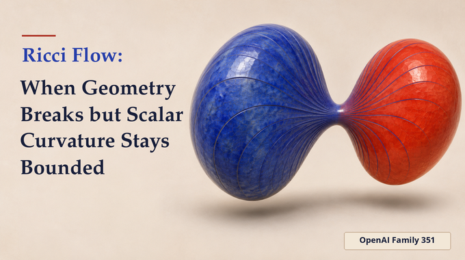
Ricci flow can reach a finite time when some sectional curvatures become arbitrarily large, even though scalar curvature stays uniformly bounded in space and time. OpenAI’s manuscript makes that split precise on a closed, sufficiently high-dimensional product of spheres. The key is a shrinking cap that sits inside a much larger region resembling a Ricci-flat cone. The cone explains why a large-scale view can miss the strongest curvature. The new estimates explain why the scalar curvature stays bounded even inside the cap, where the full curvature grows fastest.
Table of Contents
1. Ricci Flow and the Singularities Hidden in Geometry
Richard Hamilton’s Ricci flow evolves the metric , the rule for measuring lengths and angles, using its Ricci tensor. Positive Ricci curvature in a direction makes the metric shrink in that direction. The Ricci flow equation is
On a round -sphere, the squared radius falls from to . Each sectional curvature is the reciprocal of that squared radius, so the sphere becomes singular when the radius vanishes. Scalar curvature diverges there too. The paper asks whether scalar curvature must always give that warning.
1.1 The Proof in Five Stages
- Start with a singular flow. Use Stolarski’s sphere-product construction, where two radii describe an evolving geometry that approaches a Ricci-flat cone outside a small cap.
- Measure the cap. Use the gap from the cone to pin down the surviving sphere’s radius, then rule out full-curvature spikes beyond what that radius permits.
- Follow the radial drift. Move the region used for local derivative estimates with the dominant drift. The resulting estimates keep track of how the Ricci reaction term grows with dimension.
- Compare Ricci curvature with a test function. Balance diffusion against that reaction term. This isolates a power of the radius mild enough to control the source in the scalar equation.
- Bound the scalar and locate the singularity. Use an inner scalar supersolution and an exterior Ricci estimate. The shrinking sphere at the pole gives the matching lower bound on full curvature.
2. What Scalar Curvature Cannot Tell Us
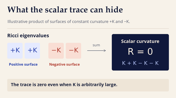
The Riemann curvature tensor, written , records curvature in tangent two-planes. Taking a trace over one pair of slots gives the Ricci tensor. Its value on a unit direction sums the sectional curvatures of planes containing that direction. Taking the trace again gives scalar curvature , a single number at each point.
For a concrete example, take the product of a surface of constant curvature and one of constant curvature . Each surface contributes two Ricci eigenvalues, so the product has eigenvalues . Its scalar curvature is zero and the sectional curvature of a plane tangent to the first surface is . Since can be arbitrarily large, the trace alone gives no pointwise bound on the underlying tensor. The question is whether this can persist along a singular flow.
3. The Scalar-Curvature Extension Conjecture
Hamilton’s extension criterion says that a smooth Ricci flow on a closed manifold extends past a finite time if its full curvature stays uniformly bounded. Šešum showed that a uniform bound on the Ricci tensor also suffices. The scalar-curvature extension conjecture asks whether a bound on the trace alone suffices in dimension four and higher.
Bing Wang’s blowup-rate restriction gives a clue about where to look. If a closed flow has a finite singular time and bounded scalar curvature, then
Thus along some sequence of times, full curvature is at least a positive constant times . This motivates looking at blowup faster than the parabolic rate.
4. What OpenAI’s Ricci Flow Proof Establishes
Theorem 1.1 gives an integer , a time , and a Ricci flow with smooth initial metric on the closed, connected manifold . The flow is smooth for and satisfies
The maximum grows beyond any fixed bound as approaches . The dimension is , and the construction needs sufficiently large. The proof gives no numerical minimum dimension for a counterexample.
OpenAI’s release describes the results as produced by an internal frontier model. The walkthrough here follows the dependencies in the written Ricci flow proof, starting with its external existence input and ending with the new curvature bounds.
5. Stolarski’s Construction and the Missing Curvature Bound
Earlier work produced Type II singularities in rotationally symmetric flows on spheres. The degenerate neckpinches of Angenent, Isenberg and Knopf, for example, exhibited different models at the tip and on the larger parabolic scale. These examples showed how a single flow could develop curvature at different length scales.
Stolarski built closed, doubly warped flows with arbitrarily fast curvature blowup and a Ricci-flat cone as the parabolic-scale model. He identified bounded scalar curvature as a possibility. A Ricci-flat cone can still have nonzero full curvature on its regular part because only the directional traces need to cancel. The cone approximation controls Ricci curvature on annuli that stay a fixed positive distance from the vertex in rescaled coordinates. The cap approaches that vertex and eventually lies inside every such annulus. The new proof uses Stolarski’s quantitative profiles and inner inequalities to reach the cap without assuming convergence to a particular cap metric.
6. Two Shrinking Scales Beneath the Singularity
Away from the poles, the doubly warped metric is
Here is radial arclength at time , the sphere metrics have sectional curvature one, and and are their metric radii. At each pole the factor collapses smoothly, with and , leaving an of positive radius for each .
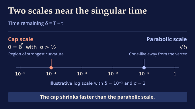
Write . The parabolic length is and the cap length is with . For intuition, if and in normalized units, these lengths are and . Their ratio tends to zero.
On fixed annuli in , the profiles control the metric through two derivatives, which gives there with for the selected modes. At a fixed multiple of , the leading inner profile keeps strictly above the cone ratio. Since its logarithmic slope is nonpositive inward of that interface in the outward radius coordinate, this fixed positive gap persists all the way in toward the pole.
7. Controlling Full Curvature Near the Collapsing Cap
The warped metric separates curvature into five kinds of sectional curvature. The radial planes with one direction in either sphere have curvatures and . Planes tangent to a single sphere use or , and mixed sphere planes use .
The first curvature-record argument bounds . If it set arbitrarily large records, rescaling at the record points would make both sphere radii huge while leaving their arclength slopes bounded. The tangential and mixed curvatures then vanish in the rescaled limit. Shi’s derivative estimates keep a remaining nonzero radial curvature of one sign over a short interval. The corresponding second derivative is proportional to the huge radius, so integrating it would force the slope outside its bounds.
The pole radius also obeys at late times. Monotonicity and the profile at the cap interface give the upper estimate. If the pole were much smaller, a long interval in logarithmic radius would force the logarithmic slope of close to one. The strict cone gap and the scalar lower bound would then force to decrease by more than its allowed range. The key here is that the proof only needs a scalar lower bound, which the ordinary maximum principle already supplies. It would be circular to assume the scalar upper bound at this stage. The negative scalar contribution from the gap can only be offset by a sustained change in the radial slope, and that change is incompatible with the construction’s slope bounds. The resulting pole estimate, together with approaching one uniformly when is small, lets a second record argument rule out unbounded . Together the estimates give
8. The Dimension-Dependent Ricci Curvature Estimate
A full-curvature bound alone gives a Ricci reaction estimate with a dimension-dependent constant. For comparison to work, the proof needs its leading coefficient. Set and . Near either pole, is a radial coordinate. The warping equations have a dominant drift . Rescaling around a fixed radius would leave a drift of order .
Instead center the cylinder at , through radius at time , and use the length . The center’s velocity cancels the dominant drift at the center. Across the cylinder, the residual involving is bounded after rescaling. One-dimensional parabolic estimates then give and , with independent of dimension and mode.
Ricci curvature has three entries up to symmetry, one radial and one for each sphere. Weight the sphere entries by the square roots of their multiplicities to make the tensor norm Euclidean. In these coordinates the curvature action is a symmetric matrix. After multiplication by , its largest eigenvalue is at most . The reaction coefficient in the Ricci norm inequality is therefore at most in the inner region. Near the pole the cap bound also gives . The diagonal entry for the directions accounts for the leading term. The derivative estimates and the mixed sphere curvatures bound the off-diagonal entries of the scaled matrix by or less. This separation matters because the comparison needs a gain proportional to , which can absorb errors proportional to . Both reaction bounds are used across the cap.
9. The Supersolution That Keeps Scalar Curvature Bounded
The Ricci comparison function is with and , where is the mode index. Its leading diffusion coefficient beats the reaction’s in sufficiently large dimension, even after the error of order . The proof fixes first and then increases the even mode so lies between zero and one. Once the flow is fixed, a small absorbs the cap reaction term. The parabolic annulus supplies the lateral data. At its inner comparison boundary, the ratio is bounded by a constant times . The dimension is chosen so , making this ratio small at late times. One multiplier then also dominates the initial data on a fixed late slice.
The positive term makes smooth at the pole at each time before , where the reaction estimate alone would be unusable. At a first interior contact with a suitable multiple of , the Ricci norm is positive and the strict differential comparison prevents it from crossing. The maximum principle gives . Since , the bound implies at positive radii in the inner region. Squaring it bounds the source in the scalar-curvature evolution equation, where is the Laplacian for the evolving metric,
Put . Applying the geometric heat operator to yields a positive multiple of , exactly the power needed to dominate the source. The proof adds a large constant and an auxiliary to compare on a region with the poles excised. It then removes the excision, sends to zero and uses continuity at each smooth time. The upper bound stays finite at the pole because . Away from the cap, a separate comparison based on bounds Ricci curvature outside a larger fixed parabolic radius. This is a smooth function across the equator, so the exterior comparison includes both hemispheres. The annular estimate joins the inner and outer regions. Together they give a scalar upper bound everywhere. The scalar minimum is bounded below by its initial value.
10. Arbitrarily Fast Type II Curvature Blowup
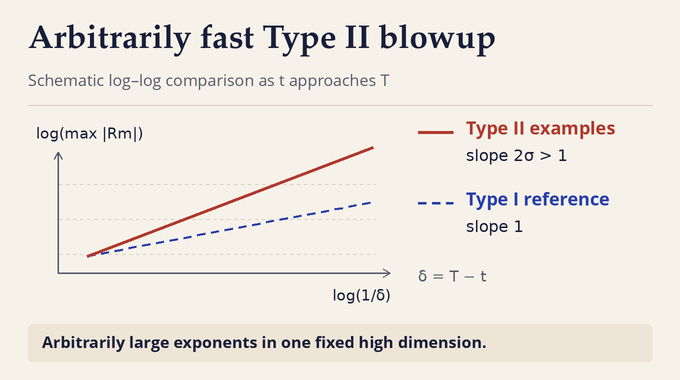
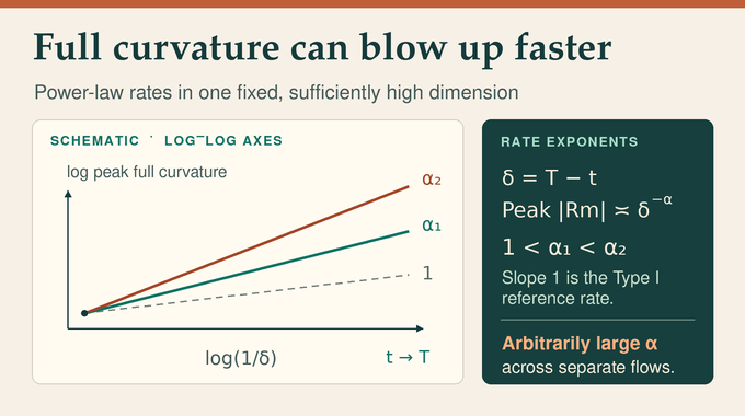
Type I permits maximum full curvature of order . In a Type II singularity the product of that maximum and is unbounded. At either pole the sectional curvature is . Since the pole radius is comparable to , this gives a lower bound matching the cap-scale upper bound.
Corollary 6.4 makes the rate precise. With and , it gives
Here means upper and lower bounds by positive constant multiples for all sufficiently late times. Fix a sufficiently large and take successively larger even . The dimension stays fixed while the exponent increases without bound. Each choice gives its own flow and comparison constants.
11. What the Counterexample Changes in Ricci Flow Theory
Bounded scalar curvature fails as a universal smooth extension criterion. In these examples, an extension on the same closed manifold would force the full curvature to stay bounded near , contrary to the pole calculation. Šešum’s criterion also implies that the Ricci tensor cannot stay uniformly bounded through this time. Smooth extension concerns this same metric family on the original manifold. Continuation in a framework that admits a singular geometry is a separate question.
The construction leaves the four-dimensional extension question open. Its lesson for Ricci flow is that a bounded trace can coexist with geometric degeneration across many power-law rates. To see what scalar curvature can still constrain, read Binary Verse AI’s analysis of scalar curvature and Urysohn width.
What is the Ricci flow equation?
Ricci flow is Richard Hamilton’s geometric evolution equation . It changes the metric in response to its Ricci tensor and can develop singularities through curvature concentration.
What is the difference between Ricci curvature and scalar curvature?
Ricci curvature is a tensor that describes directional aspects of curvature. Scalar curvature is its trace, a single number at each point. Taking the trace can hide large Ricci eigenvalues of opposite signs and loses information about individual sectional curvatures.
Can Ricci flow become singular while scalar curvature remains bounded?
Yes. OpenAI’s manuscript dated September 24, 2026, proves that a closed Ricci flow in sufficiently high dimension can have uniformly bounded scalar curvature while its maximum full curvature tends to infinity at a finite maximal time.
What is a Type II Ricci flow singularity?
At a Type II finite-time singularity, , where is the singular time. The manuscript constructs examples with two-sided power-law blowup and arbitrarily large exponents in one fixed sufficiently high dimension.
What is new in OpenAI’s Ricci flow proof?
The proof starts with Stolarski’s singular flows and adds cap-scale curvature estimates, a dimension-dependent Ricci reaction bound and a scalar-curvature supersolution. These estimates establish a uniform scalar bound up to the singular time.
Does OpenAI’s counterexample apply to four-dimensional Ricci flow?
The construction applies in sufficiently high dimensions and leaves the four-dimensional question open. Hamilton’s full-curvature and Šešum’s Ricci-tensor extension criteria still apply.