

Two D0-branes in the BFSS matrix model have a route to unlimited separation along configurations where the classical potential vanishes. Yet OpenAI’s October 2026 preprint proves that the relative Hamiltonian has infinitely many normalizable states at strictly positive energies, including a sequence of energies that tends to infinity. The escape directions remain open. In certain rotational symmetry sectors, however, a wavefunction cannot occupy the cheapest modes across those directions. The energy it must spend on transverse motion grows with separation and confines it.
Table of Contents
1. What Did OpenAI Prove About the BFSS Matrix Model?
Theorem 1.1 of the preprint gives an orthonormal sequence of square-integrable eigenvectors. Here “normalizable” means that each wavefunction has finite total probability and can be scaled to unit norm. The unbounded sequence of energies guarantees infinitely many distinct positive eigenvalues. The operator acts on gauge-invariant states after the free center-of-mass motion is removed.
The theorem is an existence result for the exact relative operator. Its proof needs only one suitable infinite-dimensional rotation sector, although the paper constructs physical sectors with arbitrarily large values of the weight coordinate used in the argument.
2. The BFSS Matrix Model and Its Connection to Quantum Gravity
Banks, Fischler, Shenker and Susskind proposed that a large-matrix limit of supersymmetric matrix quantum mechanics describes M-theory in the infinite-momentum frame. The model comes from reducing ten-dimensional supersymmetric Yang–Mills theory to one time dimension. Nine bosonic matrices describe the spatial degrees of freedom, and sixteen supercharges generate the supersymmetries. In the D0-brane picture, diagonal entries encode positions in a commuting configuration, while off-diagonal entries allow interactions between the branes.
For two branes, the matrices are . Each matrix’s trace part describes the shared center-of-mass coordinate. Once that free motion and its fermionic partners are removed, the traceless matrices describe the interacting relative system. This separation matters for what counts as binding. A state can be normalizable in the separation variables while the center of mass moves freely. The positive-energy theorem addresses precisely that internal motion.
3. Why Positive-Energy Bound States Were Considered Impossible
Far apart along a commuting configuration, the branes have zero classical potential energy. The valley extends to infinity, and in the quantum model supersymmetry makes it possible for low transverse modes and the fermionic interaction to balance. In their study of supersymmetric matrix Hamiltonians90214-9), de Wit, Lüscher and Nicolai showed that the spectrum fills and explicitly left open the question of normalizable eigenstates in that interval.
The original BFSS paper went further. In Section 5, after removing center-of-mass motion, its authors excluded additional normalizable bound states beyond the zero-energy threshold states. Danielsson, Ferretti and Sundborg later found normalizable excited wavefunctions for the same relative two-brane problem in a Born–Oppenheimer approximation. They expected decay once the approximation was lifted and described the states as metastable. An eigenstate of the exact operator would answer a stronger question. It would retain its probability distribution under the full time evolution.
4. The Mathematical Structure of the Relative SU(2) BFSS Hamiltonian
Each traceless matrix has three real coefficients in the Pauli basis. Organize the coefficients of the nine matrices into three vectors , one for each color direction. Together they form a point . “Color” refers to the internal gauge index. Spatial rotations act on the nine components of each vector, while gauge transformations rotate the three color labels and act on the fermions.
The wavefunction takes values in a finite-dimensional complex Clifford module . Its 48 fermionic generators come from sixteen spinor components in each of the three colors. A physical wavefunction is invariant under the combined gauge action on its arguments and values. On smooth, compactly supported physical states, the energy form averages the squared norms of the sixteen supercharges . The norm includes integration over the configuration space and the inner product on the fermionic module. Closing this form defines a nonnegative self-adjoint operator and specifies the domain framework for the spectral argument.
The manuscript expands the form into kinetic energy, the scalar quartic potential , and a Hermitian matrix term acting on the fermions. The kinetic term is , and the fermionic term can lower the energy. To prove confinement, the paper has to bound what the full form costs at large separation.
5. The Proof Roadmap From Escape Directions to Quantum Confinement
OpenAI attributes the release to an internal frontier model. The public release materials give no BFSS-specific discovery chronology, and the positive-energy theorem is absent from the public Lean catalogue. The numbered stages follow the written proof of Theorem 1.1.
5.1. Separate the Energy Terms
Open the sum of supercharge squares to see where energy can be gained or lost. This exposes a positive kinetic term, a quartic bosonic term and a fermionic term that can contribute negatively.
5.2. Look Across the Escape Direction
Hold one color vector fixed. Split the others into parallel and perpendicular components. The transverse coordinates feel a quadratic potential that stiffens as the fixed vector gets longer.
5.3. Identify the Rotations That Preserve the Slice
The rotations fixing the chosen vector still act on the transverse coordinates and fermions. Restrict the full rotation type to this subgroup to find which symmetry types can occur on the slice.
5.4. Remove the Cheapest Oscillator Levels
Compare the symmetry types allowed on the slice with those carried by low oscillator levels. A sufficiently large rotation weight makes the two lists disjoint, so the first several levels vanish from the wavefunction.
5.5. Turn the Excitation Cost Into Confinement
The lowest level that can contribute costs enough to overwhelm the fermionic term. Average the estimates from the three choices of color vector. The combined estimate penalizes escape in the full configuration space.
5.6. Populate a Physical Sector and Read Its Spectrum
Construct gauge-invariant states in an allowed sector and use radial variation to make the sector infinite dimensional. Confinement then forces its energy levels to form a discrete sequence that runs to infinity.
6. How Transverse Oscillators Emerge Along Flat Directions
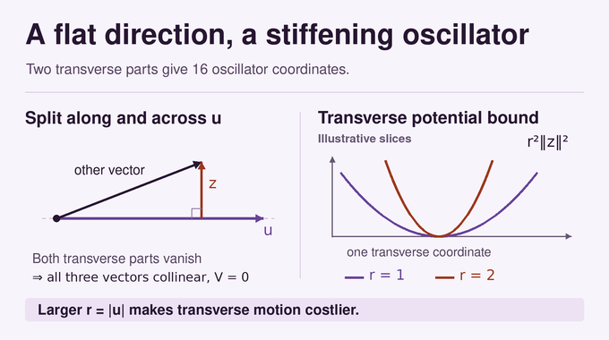
The potential is a sum of squared wedge products . Each is the squared area of the parallelogram spanned by two color vectors. All these areas vanish exactly when the vectors lie on one line. This is the commuting-matrix condition in the Pauli basis. Fix one nonzero vector . Write each of the other two vectors as , with , a real coordinate and . The pair contains sixteen real coordinates because each perpendicular space has dimension eight. Terms involving already give the lower bound in Equation (3.2).
Here is the sum of the two transverse squared lengths. For a concrete slice, take and tilt another color vector by adding . Its wedge term with is , independent of its parallel component. The same transverse displacement costs more as grows. Combining this bound with one quarter of the squared transverse gradient norm gives the comparison oscillator.
The change of variables gives a standard oscillator in sixteen dimensions, with . Its level has energy for , where eight is the sum of sixteen half-quanta. This is an exact spectrum for the comparison oscillator on a fixed slice. The proof uses those levels to bound the bosonic part of the energy form.
7. Spin(9) Symmetry and the Exclusion of Low-Energy States
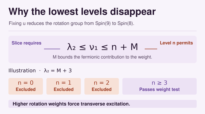
The Hamiltonian preserves the full rotation group , the double cover of . Its isotypic sector of highest weight collects all copies of the same irreducible rotation representation. Rotations preserve the closed energy form, so projecting onto a sector commutes with the resolvent of . This lets the proof treat each sector as an invariant spectral problem. The four weight coordinates encode how the representation transforms under rotations in four orthogonal planes. On a slice with fixed, the remaining rotations form a subgroup isomorphic to .
An orthogonal branching rule says that a subgroup type of highest weight can occur in the restriction of the full type only if . The paper applies this to the wavefunction on the slice by showing that restriction intertwines the subgroup actions. To bound the same weight from above, take oscillator level . Its functions are a rotation-invariant Gaussian times polynomials of degree at most . Each transverse coordinate contributes at most one to the first weight coordinate. The finite fermionic space can add at most a fixed amount . A type shared by the slice and level must therefore satisfy
The second full-group coordinate does the work because it forces a lower bound even after one spatial direction is fixed. A large first coordinate alone gives no such lower bound. If for an integer , all levels through are excluded. The oscillator projections commute with the subgroup rotations, so every excluded component is exactly zero.
In this example the first level that could contribute is , giving a lower bound of for the oscillator energy per unit squared slice norm. The inequalities establish a necessary condition on a level. Which allowed levels actually occur depends on the representation.
8. Restoring Confinement Despite the Fermionic Contribution
The fermionic matrix obeys for a finite constant , since it depends linearly on and acts in a finite-dimensional space. Its most negative possible contribution therefore grows linearly with distance. After removing levels through , the oscillator contribution on a slice is at least per unit squared norm. The proof integrates that estimate over the fixed coordinates, then averages it over the three choices .
The sum of the three color-vector lengths is at least . This gives a net coefficient , made positive by choosing large enough and then taking . A quarter of the gradient energy remains available. The resulting bound from Proposition 3.4 holds on the closed form domain in the selected sector.
The gradient controls oscillations on bounded regions. The weighted integral limits the squared norm outside a ball of radius to . Together, local Rellich compactness and this uniform tail estimate make the inclusion of the form domain into the sector Hilbert space compact. The resolvent is compact because it maps bounded sets into bounded sets in the form domain. Also, a zero-energy vector would have vanishing weighted norm and so would be zero, since is positive almost everywhere.
9. Constructing Infinitely Many Normalizable Positive-Energy States
A weight cutoff would prove little if no physical states carried those weights. The paper first pairs the fermionic generators into annihilation and creation operators. Gauge rotations preserve the one-dimensional vacuum line annihilated by all annihilation operators. Since has no nontrivial continuous one-dimensional character, the vacuum line is gauge invariant. The space of gauge-invariant fermionic vectors is also rotation invariant, so the paper can choose a highest vector of some rotation weight there.
The spatial factor is a gauge-invariant polynomial . Take two complex vectors in the first two rotation planes and , and write and using bilinear dot products. The polynomial sums the squares of the two-by-two minors.
The sum is a Gram determinant in the color variables, hence gauge invariant. Each minor inherits the highest weight of the bivector . Multiplying by raises each of the first two weight coordinates by . Multiplication by a smooth function supported in a radial shell preserves that rotation type. Arbitrarily many disjoint shells give independent vectors in the same sector, because is nonzero somewhere on each shell.
Now choose so the sector meets the confinement threshold. A nonnegative operator with compact resolvent on this infinite-dimensional sector has an orthonormal eigenbasis with energies tending to infinity. The kernel calculation gives strict positivity. Since the sector reduces , these are eigenvectors of the full physical Hamiltonian.
10. Bound States Inside a Continuous Spectrum and the Apparent Paradox
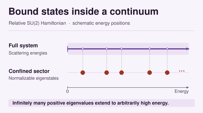
An interval filled by scattering energies can contain eigenvalues. Scattering states can carry probability to large separations. A point-spectrum state has a square-integrable eigenvector, and its time evolution multiplies its wavefunction by a phase, leaving its probability distribution fixed. The new eigenvalues are discrete within their sectors and embedded in the full spectral set. In the full system, there are other spectral energies arbitrarily close to each of them.
Rotation symmetry explains how both behaviors fit the same Hamiltonian. Time evolution stays in the initial symmetry sector, and the sectors constructed in the paper have compact resolvent. Scattering channels in the full system therefore offer no decay route for these exact eigenstates. The result makes no assertion about their stability under perturbations that break the symmetry. It also coexists with the unique zero-energy state reported in OpenAI’s companion threshold preprint. That claim concerns the kernel, while the new tower lies above zero.
11. What the Discovery Means for M-Theory and What Remains Unsolved
The original exclusion of extra normalizable states fails already for two D0-branes. The BFSS conjecture about recovering M-theory in an appropriate large- limit remains open. This finite- theorem gives neither individual energy values nor a classification of every sector. Larger matrices have more ways to split into widely separated clusters, and the paper leaves open whether analogous bound states occur at larger matrix sizes.
The BFSS matrix model offers a precise lesson about quantum escape. A flat classical potential gives the branes a route to separate, but the symmetry of a wavefunction determines whether it can afford the transverse motion along that route. Follow Binary Verse AI for more research explainers on Yang–Mills existence, chiral gauge theory, the Hawking–Page transition and quantum spin systems.
What is the BFSS matrix model?
The BFSS matrix model is a supersymmetric matrix quantum mechanical system proposed as a nonperturbative description of M-theory. Its matrix degrees of freedom describe interacting D0-branes, with a proposed connection to eleven-dimensional physics in an appropriate large-N limit.
What did OpenAI prove about the BFSS Hamiltonian?
OpenAI proved that the relative SU(2) BFSS Hamiltonian has infinitely many strictly positive eigenvalues with square-integrable eigenvectors. The energies include a sequence tending to infinity, overturning the original paper’s exclusion of normalizable positive-energy bound states for N = 2.
Why are positive-energy bound states surprising in the BFSS model?
The classical potential vanishes on commuting-matrix configurations, leaving routes to arbitrarily large separation. In selected rotational symmetry sectors, the lowest transverse oscillator modes are forbidden. The remaining modes cost more energy as the branes separate and confine those sectors.
Can bound states exist within a continuous energy spectrum?
Yes. An energy in the scattering continuum can also be an eigenvalue with a square-integrable eigenvector. The BFSS proof finds such eigenvectors in confined rotational sectors while the full Hamiltonian still allows scattering.
Does the OpenAI proof contradict the unique BFSS ground state?
No. Ground-state uniqueness concerns normalizable states at exactly zero energy. The eigenstates shown to exist in the positive-energy paper have strictly positive energies, so the results are compatible.
Does the discovery disprove the BFSS conjecture or M-theory?
No. The theorem overturns an assertion about positive-energy bound states of the relative SU(2) Hamiltonian. The large-N conjecture and the existence of analogous bound states at larger matrix sizes remain open.