
An exact copy of the distances among a set of points can need quadratically many coordinates, even when the points themselves number only in the dozens. Allow a fixed amount of distortion, however small, and OpenAI’s preprint proves that the worst-case dimension drops below every positive power of the point count. This is dimension reduction in Lp with the geometry kept intact up to a multiplicative factor. The map chooses new coordinates while keeping the same norm exponent. The proof works by matching the moments of random pairwise differences while keeping those differences consistent with a single set of point labels.
Table of Contents
01. What Is Dimension Reduction in Lp, and Why Is It Difficult?
Take distinct points from a real space. In the function-space setting, the distance between two points is the th root of the integral of their absolute difference raised to the th power. The finite target uses the same rule with a sum over coordinates. The source can be infinite-dimensional. The embedding must preserve all pairwise distances within the same distortion allowance.
| Item | What the theorem covers |
|---|---|
| Source and target | Finite subsets of real into with the same exponent |
| Exponents | with in Theorem 1.1 |
| Fixed distortion above one | Subpolynomial dimension |
| Exact distances | Quadratic worst-case dimension for the same non-Euclidean exponents |
| Map | Unrestricted on the finite set and allowed to be nonlinear |
A single vector assignment must serve both short and long pairs. A small additive error can overwhelm the distance between two close points, so the guarantee controls relative error for every pair after one global rescaling. A separate question in metric geometry, covered in our Falconer distance explainer, asks what distances a set determines. Here the entire list of distances, with the pairs identified, is the input to preserve.
02. The Johnson–Lindenstrauss Lemma and the Problem Beyond Euclidean Geometry
For , the Johnson–Lindenstrauss lemma gives dimensions at any fixed distortion . Euclidean distances come from an inner product, and random linear projections can concentrate the squared norm of each difference vector. Taking a union bound over pairs then gives a simultaneous guarantee.
Asking for a Johnson–Lindenstrauss lemma in Lp raises two choices. One concerns the target, which here must use the original exponent. The other concerns linearity. A linear map must respect relations among the source vectors. Nonlinear Lp embeddings can position the points independently of those relations, subject to the distances. For another kind of metric guarantee, see our coverage of edit distance approximation.
03. The Previous Limitation and What the Earlier Lp Bounds Left Open
Ball’s work established the pair-count upper bound for exact embeddings and showed that quadratic order is necessary when . Below two, Schechtman’s approximate finite-set estimates went from to . Linear subspace discretization addresses a different parameter, the dimension of a subspace whose entire norm structure must be preserved. The span of the translated data can have dimension , so a bound in that parameter alone gives no subpolynomial guarantee in .
Selected configurations already force dimension proportional to the number of points when the map must be linear and . The new theorem answers the open question of whether free placement in same-exponent coordinates permits sublinear dimension at fixed distortion.
04. OpenAI’s Subpolynomial Dimension Reduction Theorem Explained
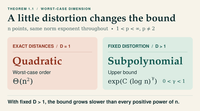
For Theorem 1.1 in the September 23, 2026 preprint, write as the least dimension that works for every -point subset of every real space. For a given set, the images of the source points must satisfy the following inequalities for every pair, with one scale .
In this definition of Lp embedding distortion, the largest target-to-source distance ratio can be at most times the smallest. For fixed , , and , the theorem gives
All unmarked logarithms are natural. The exponent is below two and above two. For , subtracting from two gives . For , subtracting from one also gives . Both upper bounds therefore have a square root of in the exponential. The constants can differ and may grow as distortion approaches one.
05. Why Exact Embeddings Face a Quadratic Obstruction
Each scalar coordinate contributes a vector of powered pairwise distances. Divide each nonzero contribution by the sum of its entries. These normalized vectors lie in an affine hyperplane of dimension at most . The normalized total distance vector is a barycenter of this compact set, even when the original distances come from integration. Carathéodory’s theorem represents it with at most contributions. Rescaling their coordinate labels realizes the original distances exactly.
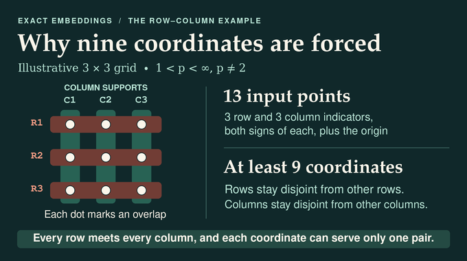
For the lower bound, take the positive and negative indicators of every row and column of a grid, plus the origin. In any isometric image fixing the origin, strict convexity forces antipodal points to remain antipodal. This makes the norms of sums and differences recoverable from the distance list. For two real coordinate entries and , the -parallelogram defect is
For , it vanishes exactly when and otherwise has the sign of . Across coordinates, nonzero defects cannot cancel. Distinct rows thus retain disjoint supports, as do distinct columns. Each row and column must still overlap, since their defect is . Each target coordinate witnesses at most one row–column intersection, so points require at least coordinates. In the case, thirteen points force nine coordinates. For general , take and pad the configuration with distinct points if needed. Any exact embedding of the padded set must still realize the original intersections. This is a dimension obstruction tied to exact distances, distinct from the covering-based notion in our Urysohn width explainer.
06. The First Proof Step and the Role of Normalized Gradients
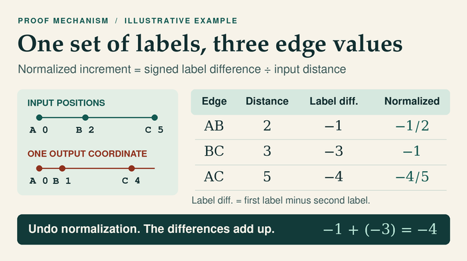
View the points as vertices of a complete graph and orient each edge once. For an edge , let . One output coordinate gives each vertex a scalar label . Its normalized increment is . The subspace consists of all edge vectors obtained in this way. Fixing one label at zero makes recovery of the remaining labels unique.
For example, on the real line take input positions zero, two, and five and candidate labels zero, one, and four. The normalized increments along edges , , and are , , and . Multiplying back by the input distances gives , , and , with the first two summing to the third. Changing only the last increment can break that consistency. Sampling vectors in gives coordinates that always fit together.
07. How Weighted Moments Control Every Pair
Lemma 3.1 asks for a random gradient whose largest absolute entry is at most almost surely. For every strictly positive probability weighting of the edges, the proof can choose a distribution with weighted absolute moment error at most , where is the target th moment and is a small tolerance. Both and must stay fixed across tests. The criterion is
where is the set of edges and denotes expectation.
Mixing distributions gives a compact convex set of moment vectors. If it missed the box of vectors within of on every edge, a separating hyperplane would supply a failed weighted test. The proof uses the absolute values of the separating coefficients, with a uniform component to make every weight positive. One law thus meets all edge targets.
Independent draws now supply coordinates, with the recovered labels scaled by . The powered distance ratios are sample averages of values in . A bounded-sum estimate and a union bound over the pairs give a sufficient dimension of order . The resulting distortion is at most .
08. Electrical-Flow Localization and the Logarithmic Projection Bound
Clipping edge values individually can break the consistency illustrated above. To restore it, the proof projects onto using a weighted least-squares norm. For each test , the paper chooses a probability weighting with . In the weighted quadratic norm, both the projection and its residual are contractions.
With conductances , the projection is equivalent by diagonal rescaling to an electrical-flow projection. The localization theorem of Gurel-Gurevich, Nachmias, and Sachdeva bounds the Euclidean operator norm of the entrywise absolute projection matrix. This controls a weighted quadratic average of the absolute row sums of . A continuous reweighting allocates more mass to large rows. Brouwer’s fixed-point theorem supplies weights for which every row sum is at most . The quadratic norm controls average error, while the row bound limits the largest entry after projection. The localization argument uses the graph heat kernel, a continuous-time random walk. Random walks serve a different purpose in the switch-chain mixing proof, where the question is how quickly a sampler approaches equilibrium.
09. Homogeneous Increments and Signed Poisson Sampling
The proof can start with finitely many input coordinates by exact discretization. It divides each coordinate difference by the original pairwise distance and multiplies the resulting gradient by a positive scale . On each source coordinate the scale carries intensity . Because the powered normalized differences sum to one for each edge, the resulting measure satisfies for every edge and every . This is an intensity measure. Its total mass can be infinite.
On a finite-mass region, take a Poisson number of independent jumps with mean equal to that mass and attach independent random signs. Their sum has mean zero and, for bounded jumps, variance equal to the integrated squared jump size. The magnitude density makes that integral finite near zero below two and finite near infinity above two. This common law is marginal. Edges can be dependent because a single jump labels all vertices.
10. The Proof for 1 < p < 2 Using Stable Distributions and Clipping
Below two, the sum of small jumps converges in quadratic mean across dyadic bands. Adding the finite Poisson sum of large jumps gives a gradient with common symmetric -stable marginals. Their tails have order for , so the full th moment diverges logarithmically. Capping the magnitude at gives a common finite moment that grows on the order of .
The paper clips each entry of at magnitude , projects back to , and compares the projected moments at the smaller level . The row bound controls the expected clipping error after projection. Weighted quadratic contraction controls the part of the projected th moments above the cap. At this choice of , the combined weighted error is of order at most . Taking to be a sufficiently large multiple of makes the error small relative to . The resulting magnitude bound has .
11. The Proof for p > 2 Using Overlapping Truncations
Above two, the construction sums overlapping dyadic bands. Band keeps magnitudes in for . The number of bands covering a magnitude rises from one to and then falls back to one. Each dyadic bin contributes times its multiplicity to the power . The common integrated th-power magnitude therefore has order .
Projection repairs the truncated increments. The paper estimates the repair at each cutoff in two ways. The retained low-magnitude part bounds the maximum size of the repair. Since the original gradient already lies in , the repair can also be written using only the discarded high-magnitude part, which has finite quadratic energy. Splitting at the appropriate cutoff gives a tail bound for the total repair. Its error, measured as a weighted integrated th power, is at most of order . The ratio of the error norm to the input norm is thus at most a constant times . Choosing to be a sufficiently large multiple of makes the relative error small.
Signed Poisson sampling then turns the projected jumps into random gradients. The paper’s nearly additive moment estimate bounds the sampled th moment by the integrated th power with leading coefficient as close to one as needed, plus a variance term. That leading coefficient matters when the allowed distortion is close to one. The proof discards an entire draw if any entry is too large, preserving consistency. This gives .
12. Completing OpenAI’s Proof and Identifying the Open Questions
The moment criterion turns either bound on into a bound of the same order on . Since , dividing by gives a quantity tending to zero. That is the meaning of here. Exact discretization covers the finitely many small sizes outside the asymptotic estimates.
For the packing lower bound, start with the equilateral set of coordinate unit vectors. Translate and scale the images so that they are one-separated and lie in a ball of radius . The open half-unit balls around them are disjoint and lie inside a ball of radius . Volume scales as the th power of radius, so , giving the theorem’s logarithmic lower bound.
| Regime | Worst-case dimension guarantee |
|---|---|
| , | Logarithmic order for fixed distortion |
| , | Subpolynomial upper bound and logarithmic packing lower bound |
| , | Between and for |
At , Brinkman and Charikar give obstructions even for nonlinear maps. Above two, the stronger lower bound of Naor and Ren rules out a universal logarithmic guarantee at fixed distortion. Along arbitrarily large cardinalities it gives at least order coordinates. The preprint leaves the optimal growth rate and efficient construction open, so it gives no runtime guarantee for applications such as metric k-median.
OpenAI’s release announcement describes the broader collection. The Lean scope note for family 094 documents the approximate and exact bounds, attainment of the least dimension, and both asymptotic limits. The Lean theorem file is the formal counterpart to those claims. For another formalization in the release, see our weak and strong normalization explainer. Binary Verse AI’s coverage of OpenAI’s mathematical proofs puts this result in the context of the wider release.
Dimension reduction in Lp now has a sharp qualitative dividing line. At exact distortion, support intersections can force quadratic dimension. With any fixed tolerance above one, consistent random coordinates can preserve every pair in subpolynomial dimension. Follow Binary Verse AI for more paper-led explainers on the boundary between geometric constraints and approximation.
What is dimension reduction in Lp?
It represents finitely many points from a real Lp space in fewer ℓp coordinates while approximately preserving every pairwise distance. The exponent p stays the same.
How many dimensions does OpenAI’s proof require?
For each fixed p strictly between one and infinity, excluding two, and each fixed distortion D greater than one, the worst-case dimension is subpolynomial in the number of points. The upper bound is exponential in a constant times the γ(p)th power of the logarithm of n, where γ(p) is 2 minus p below two and 1 minus 2 divided by p above two. The constant depends on p and D.
Why can a small distortion reduce the dimension so dramatically?
Exact distances enforce geometric relationships, including which coordinate supports must intersect. Those relationships can require quadratically many coordinates. Allowing any fixed distortion greater than one lets the proof approximately match the moments of pairwise differences instead.
How does this proof differ from the Johnson–Lindenstrauss lemma?
The Johnson–Lindenstrauss lemma gives logarithmic dimension for Euclidean geometry at fixed distortion. OpenAI’s result covers exponents strictly between one and infinity other than two, allows nonlinear embeddings, and gives a subpolynomial upper bound.
Why does the proof use different methods for p below and above 2?
Below two, the small jumps have finite integrated second moment, and the proof clips symmetric stable marginals before projecting. Above two, the large jumps have finite integrated second moment, and the proof uses overlapping truncations and signed Poisson moment estimates.
Does the theorem also work for L1 spaces?
The theorem applies for p strictly greater than one. At p equal to one, known lower bounds rule out a universal subpolynomial guarantee at fixed distortion, even for nonlinear maps.
Does OpenAI’s proof provide an efficient algorithm or optimal dimension bound?
The paper proves that the embeddings exist. It leaves efficient construction and the optimal dimension bound open.