
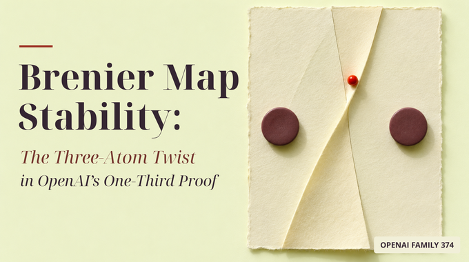
How can moving a tiny amount of probability mass cause a much larger change in the optimal transport map? OpenAI’s Brenier map paper answers with three target atoms. Keep two atoms fixed and move the lightest one sideways. The target distribution barely changes, yet a thin region of the source gets reassigned to destinations roughly one unit apart.
OpenAI proves that for a fixed uniform convex source in dimension at least two, the root-mean-square distance between maps is bounded by a constant times the cube root of the targets’ 2-Wasserstein distance. The three-atom example attains that scale and disproves Cyril Letrouit’s conjectured uniform square-root bound. The distances pair points in different ways. The target distance can choose the cheapest matching between destinations, while the map distance compares where the same source point goes.
Table of Contents
1. What Is a Brenier Map, and Why Does Its Stability Matter?
In quadratic optimal transport, a source distribution must be sent to a target distribution . A map does this when its pushforward equals . Drawing from and reporting gives a sample with law . The optimal map minimizes the average squared travel distance among maps with that pushforward.
For the source here, Brenier’s theorem identifies the optimal transport map as almost everywhere, where is convex. The map is unique up to source-null sets, and adding a constant to the potential leaves the map unchanged. For a target made of atoms, the gradient is piecewise constant. Stability asks how much those assignments can change when the target law changes.
| Topic | Paper’s Result |
|---|---|
| Source | Uniform probability on a compact convex body with nonempty interior in dimension at least two. |
| Targets | Borel probability measures in one fixed, nonempty compact set. |
| Sharp Rate | One-third Hölder stability from target distance to map distance. |
| Sharpness Example | Three atoms on a fixed cube. One moves and two stay put. |
| Main Proof Step | Linear control of the potentials, followed by interpolation for their gradients. |
2. The Original Problem: How Much Can an Optimal Transport Map Change?
Take compact and convex with nonempty interior, and put , where is its volume. Fix a nonempty compact set containing both targets. A coupling is a joint law of target points with marginals . Define the target and map distances as follows.
Here is the set of all such couplings. For the second distance, the pairing is prescribed by the two maps evaluated at the same . Those evaluations themselves induce a target coupling, so their root-mean-square disagreement is at least $W_2(\mu, u)$. The difficult direction is bounding it from above by a modulus that works across all pairs in the container. A bound that deteriorates as an atom loses mass cannot answer that uniform question.
3. Previous Stability Bounds and the Square-Root Conjecture
Earlier work on optimal transport stability often used , the minimum mean travel distance. Delalande and Mérigot obtained a map bound for source densities bounded above and below on a convex domain and targets in a fixed compact set. The manuscript also cites a sharp result by Mérigot. The inequality transfers a quarter-power upper bound to with the same power. It gives no route by itself to the stronger cube-root rate at small distances.
Earlier work by Mérigot, Delalande, and Chazal also obtained a dimension-independent exponent of in for a uniform convex source. At the other end of the regularity scale, the paper cites a Lipschitz bound in for uniformly positive Hölder densities on suitably regular, uniformly convex domains. Such density assumptions remove the light atoms that drive the cube example.
Divol, Niles-Weed, and Pooladian had already proved a estimate for regular sources and nondegenerate finite targets, with constants depending on features such as minimum atom mass and site geometry. Letrouit found an obstruction to exponents above one-third for a nonconvex source and conjectured that uniform square-root stability would hold for a uniform convex source. The cube example tests that conjecture with convexity fully in place.
4. OpenAI’s Main Theorem: Sharp One-Third Hölder Stability
Theorem 1.1 of OpenAI’s September 25, 2026 manuscript, Sharp One-Third Stability of Brenier Maps, fixes an integer , a compact convex body with nonempty interior, its uniform law , and a nonempty compact target container . There is a finite constant such that for all Borel probability measures supported in ,
The constant can depend on the geometry of the source and an enclosing radius for the targets. The stability of optimal transport maps is uniform across arbitrarily small positive atom masses, arbitrarily close sites, and targets with or without densities. The source body may have flat faces, and the compact target container may be nonconvex. The upper bound guarantees the cube-root rate across the class. Sharpness asks whether any larger exponent can work with one finite constant. Proposition 2.2 answers it on a single fixed cube in every dimension covered by the theorem.
5. The Three-Atom Counterexample: A Small Tilt With Large Consequences
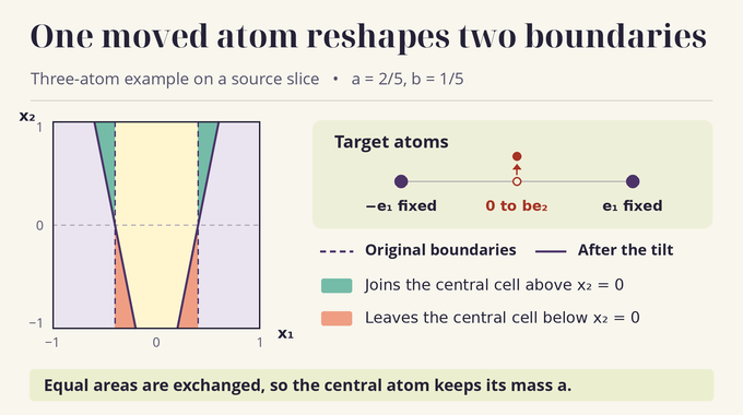
Set . Write for the first two coordinate unit vectors, take , and put . The paper compares two convex potentials, each a maximum of three affine functions.
Their gradients are optimal maps to their own pushforwards, by Lemma 2.1. The outer planes have slopes and . The middle plane has slope before the tilt and after it. The central Laguerre cell, where that plane wins, changes from to , ignoring null boundaries.
On the slice , the conditional central mass changes from to . The positive and negative contributions cancel because is uniform on . The central weight therefore remains and the two outer weights remain each. Call the original and tilted target laws and . Above the midline the central cell takes points from the outer cells. Below it the central cell gives points back.
6. Why the Three-Atom Example Rules Out Every Exponent Above One-Third
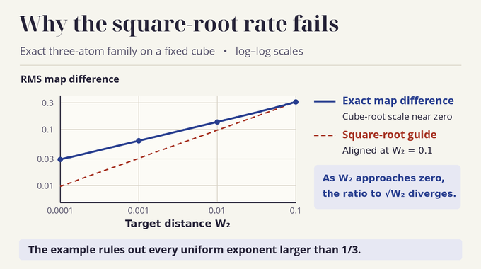
On the target side, fix both outer atoms and send mass from to . The squared cost is . Every origin in the first target has second coordinate zero, and the second target puts mass at second coordinate . That coordinate alone forces squared cost at least in any coupling. Hence .
On the source side, write for points in exactly one of the central cells. The intervals on any slice are nested, so the conditional mass in their symmetric difference is . Integrating against the uniform law of gives . The map difference has first coordinate of magnitude one there and zero elsewhere. Its second coordinate has magnitude throughout , whose mass is . The coordinate contributions add as squares, giving . Substituting yields the exact distances.
The ratio of map distance to is . It diverges as tends to zero whenever , including . The number of atoms and the cube stay fixed. In this same family , so the map distance has quarter-power scaling in and cube-root scaling in .
7. Laguerre Cells, Convex Potentials, and Prescribed Cell Masses
The positive proof begins with finite targets. For distinct sites , let with intercepts . The cell is the part of where the th affine function wins. Its mass is and its first moment is . The moment includes the mass, so the cell centroid is for a positive cell.
If two cells meet at a face , changing their relative intercepts moves the separating plane. The mass derivative on that face is weighted by , where denotes surface measure. For moments the corresponding coefficient integrates over the face with the same normalization. Lower-dimensional contacts contribute zero. The fixed-site mass derivative in direction is the weighted graph Laplacian .
Positive cells form a connected face graph. The Laplacian has only constant vectors in its kernel and its range is the zero-sum vectors. For prescribed positive masses summing to one, minimizing a convex objective gives intercepts with . Fixing removes the common additive shift. The implicit function theorem then gives differentiable intercepts as distinct sites move.
Changing a site adds a term proportional to to the face motion for site velocities . It gives the face’s first moment a second role. The coefficient that measures how an intercept change alters a cell moment also appears when site motion changes the mass. This symmetry is what later links the fixed-site estimate to the moving-site problem.
8. The Uniform Cell-Moment Estimate: The Proof’s Key Innovation
The proof now fixes the sites and varies the intercepts in direction . Let dots denote derivatives in that direction and choose so lies in the ball of radius centered at zero. Lemma 4.1 bounds the first-moment derivatives by the mass derivatives with an absolute constant .
Compare each cell at intercepts and . If and are sampled from those two cells, their midpoint lies in the original cell because the intercept perturbations cancel in the affine inequalities. The coupling uses Knothe’s triangular rearrangement to draw the two points using the same sequence of conditional quantiles. The arithmetic–geometric mean inequality on the diagonal derivatives of the midpoint map bounds its density. After weighting by the geometric mean of the two perturbed masses, the midpoint law is dominated by the restriction of to the original cell.
Testing this domination with produces a squared displacement term . Summing over the cells makes the endpoint integrals reduce to integrals on the whole source. The paper bounds the remaining terms by weighted squared mass changes and controls the moment differences before taking the derivative limit. The permitted step size can depend on the smallest mass. The resulting constant 162 is independent of cell count, masses, and site separation.
The gap between the arithmetic and geometric means of the two masses scales as their squared difference divided by the original cell mass. A Cauchy–Schwarz estimate absorbs the term coupling displacement to mass change.
9. Moving Target Atoms Without Losing Uniform Stability
Choose an optimal coupling of the finite targets and label its distinct pairs by . Each carries mass and moves at velocity along the segment between its two sites. Write , so . Swapping equal portions of two paired masses would improve the coupling if their endpoint differences had negative inner product. This nonnegative inner product keeps the segments’ moving sites distinct at every interior time, even when sites coincide at an endpoint.
Choose the normalized intercepts to keep each cell at its coupling mass and write . Since , the Laplacian range supplies an intercept direction with . Testing the differentiated mass constraints against that direction gives
Here is the first-moment derivative in the intercept direction with sites fixed. Weighted Cauchy–Schwarz and the cell-moment bound give .
The implicit function theorem provides differentiability for each particular configuration. The estimate used for stability comes from the mass-weighted calculation above. It requires no uniform bound on the inverse Laplacian, even when small cell faces make its weights poorly conditioned.
10. From Convex Potential Stability to the Sharp One-Third Exponent
On the active cell, the time derivative of the moving potential is . The velocity estimates bound its norm by . Each intercept has a finite endpoint limit, and the endpoint maxima give the maps to the original targets, with repeated slopes merged. Integrating the derivative bound over the unit time interval gives
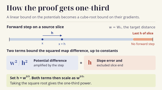
To turn this into a map bound, intersect the source with lines parallel to each coordinate axis. Convexity makes each nonempty slice an interval and makes the directional derivatives monotone along it. A forward difference over a length costs a factor in squared norm. The monotone derivative error and the terminal portion of the slice, where the forward step leaves , together cost a multiple of . Summing the slice estimates gives
Here bounds the target radii and sums the -dimensional volumes of the coordinate projections of . For , choosing puts both terms at scale . Taking the square root gives the one-third exponent. When , the targets coincide and uniqueness gives identical maps almost everywhere.
The sharpness family also checks the potential estimate. After subtracting the common weighted intercept mean, the paper computes $\lVert u_a- ilde{u}_a Vert_{L^2( ho)}^2=(5/16)W_2(\mu_a, u_a)^2$. Thus in this example the loss in exponent occurs when comparing the gradients. The values of the potentials themselves already obey a linear rate.
11. From Finite Targets to General Measures: Proof Scope and Lean Verification
For any target law on , send each point to a nearest point of a finite -net in , breaking ties by a fixed ordering. Each such discretization costs at most in . The uniform finite-target bound makes the associated maps Cauchy in as the mesh tends to zero. Supporting inequalities for the convex potentials pass to the limit and identify its gradient as the unique optimal map. The same constant thus applies to discrete, singular, and absolutely continuous targets.
Using the same net for both targets increases their mutual distance by at most twice the mesh radius. This follows by taking any coupling of the original laws, rounding each point in the pair through the same selection, and applying the triangle inequality for the root-mean-square cost. Passing to the limit preserves the estimate for the two limiting maps.
OpenAI’s release announcement describes the broader research program. Its Lean scope note for family 374 reports formal proofs of the uniform one-third estimate and the fixed-cube obstruction for every larger exponent. The Lean comparator statements specify the hypotheses and the two conclusions that the proof modules are checked against. The theorem controls disagreement between exact optimal maps. Rates for nonuniform or changing sources require separate hypotheses. Solver runtime and numerical error are separate questions.
The Brenier map result explains how a vanishing target atom can still drive a substantial change in assignments. The linear control of the potentials survives that degeneration, while the cube geometry shows exactly how much can be lost when passing to their gradients. Follow Binary Verse AI’s coverage of AI-assisted mathematical proofs, including the role of convexity in the logarithmic Brunn–Minkowski proof and the use of Lean in the formalization of Fermat’s Last Theorem.
What is a Brenier map in optimal transport?
A Brenier map is an optimal transport map given by the gradient of a convex potential. For quadratic transport from the uniform source in this paper, the optimal map is unique almost everywhere.
What does one-third Hölder stability of Brenier maps mean?
The root-mean-square difference between the two optimal maps is bounded by a constant times the cube root of the targets’ 2-Wasserstein distance. The same constant works for all target distributions supported in the same fixed compact set.
Why does OpenAI’s proof disprove the square-root stability conjecture?
The paper constructs pairs of three-atom targets whose map distance scales as the cube root of their 2-Wasserstein distance. As the target distance approaches zero, the ratio of the map distance to any target-distance power above one-third diverges. That includes the conjectured square-root rate.
Why are only three target atoms enough to prove sharpness?
A family of three-atom examples on a single fixed cube rules out every larger uniform exponent. One light atom moves while the two outer atoms stay fixed. The tilt reassigns some source points between destinations a unit or more apart.
How does the proof obtain the one-third exponent?
The paper first bounds the root-mean-square difference between normalized convex potentials linearly in the 2-Wasserstein distance. A gradient interpolation inequality then converts potential control into map control. Balancing its two terms yields the exponent one-third.
Does the stability theorem apply to discrete, singular, and continuous distributions?
Yes. The theorem covers all three types of target distributions when their supports lie in a fixed nonempty compact set. The source must be uniform on a compact convex body with nonempty interior, in dimension at least two.
Has OpenAI’s one-third stability proof been formally verified in Lean?
OpenAI’s published Lean scope note reports formal proofs of both the uniform one-third stability estimate and the sharpness counterexample. That report concerns the theorem statements. Independent expert review of the accompanying manuscript is a separate process.