
A group can have a length-two free resolution and still need a three-dimensional classifying space. OpenAI’s September 2026 manuscript proves that this happens for a finitely generated, residually finite group, giving a counterexample to the Eilenberg Ganea conjecture. The proof turns on a test with unit quaternions. Assign each edge of an acyclic complex a quaternion arbitrarily close to the identity. The ordered product around every triangle is exactly the identity, yet a longer closed path can have a nontrivial product. OpenAI proves that the existence of a two-dimensional classifying space would force every closed-path product to be trivial.
Table of Contents
1. Eilenberg–Ganea Conjecture: Why Was Dimension Two the Exception?
In 1957, Eilenberg and Ganea established equality between integral cohomological dimension and geometric dimension when the former is at least three and finite. Dimension one is covered by the Stallings–Swan theorem, which characterizes groups of integral cohomological dimension one as free. Dimension zero gives the trivial group. In dimension two, the classical bounds allowed the geometric dimension to be either two or three.
| Property | Result |
|---|---|
| Integral cohomological dimension | 2, attained by a length-two free resolution |
| Geometric dimension | 3, with all two-dimensional models excluded |
| Construction | Height kernel in a right-angled Artin group |
| Group properties | Finitely generated, residually finite, and of type FL |
| Finite presentation | Excluded for this group by the Bestvina–Brady criterion |
2. Cohomological vs Geometric Dimension: Why Can They Disagree?
Let be a discrete group and its integral group ring. The integral cohomological dimension is the shortest length of a projective resolution of the trivial module , on which every element of the group acts as the identity. A resolution is an exact sequence of modules ending in . Exactness says that everything killed by one map comes from the preceding map. Projective modules are direct summands of free modules, and a free resolution is a special case.
The geometric dimension is the smallest dimension of a connected CW complex with fundamental group and contractible universal cover. This classifying space is an Eilenberg–Mac Lane space of type . Lifting its cells gives free group-ring modules, whose augmented chain sequence is exact by contractibility.
A torus illustrates how the two measures can agree. Its universal cover is a plane, so it gives a two-dimensional model for . Its nonzero second integral cohomology requires a resolution of length at least two. The counterexample exploits the gap between filling cycles as chains and contracting loops by homotopy.
3. The Bestvina–Brady Construction and the Missing Proof
In 1997, Bestvina and Brady used height kernels to separate homological and homotopical finiteness properties. Their two-dimensional acyclic examples supplied candidates for the Eilenberg–Ganea problem. For suitable triangulations of a spine of the Poincaré homology sphere, they proved that at least one of the Eilenberg–Ganea and Whitehead conjectures fails. Whitehead’s conjecture asks whether every connected subcomplex of an aspherical two-dimensional CW complex is itself aspherical.
That alternative left the geometric dimension of the candidate unresolved. The new proof retains the height-kernel construction and adds a way to test the relators of an arbitrary aspherical presentation.
4. The New Theorem: A Finitely Generated Group With Two Different Dimensions
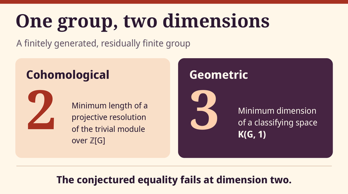
Theorem 1.1 of OpenAI’s manuscript constructs a finitely generated, residually finite group with the following dimensions.
Residual finiteness means that each nonidentity element survives in some finite quotient. Finite generation gives a finite alphabet for describing group elements, whereas finite presentation would also require a finite list of defining relations. The seed complex has nontrivial fundamental group, so the Bestvina–Brady finite-presentability criterion rules out finite presentation for this group. Its length-two resolution nevertheless has finitely generated free modules, making it type FL and hence type .
5. Building the Seed: An Acyclic Complex With Quaternion Monodromy
The seed has one vertex, two loop edges , and two discs attached to impose these relations.
For the first attaching word, the signed totals of are . For the second, the three inverse copies of give totals after including . With these vectors as rows, the exponent-sum matrix has determinant . Thus the cellular boundary from dimension two to dimension one is an integral isomorphism. The complex is acyclic because the edges are loops at one vertex and there are no cells above dimension two.
The same relations retain information about the order of multiplication. Identify with the group of unit quaternions, let , and choose imaginary unit quaternions whose Euclidean dot product is . This is possible because . The representation sends to and to . Both and map to . The image of has real part , so its cube is also . The image of is an imaginary unit and therefore differs from the identity.
To obtain the finite flag complex , the paper subdivides the loop graph, cones the attaching polygons while keeping radial edges distinct by boundary occurrence, and takes the order complex of the resulting regular cells. Pairwise comparable cells form a chain, which makes this triangulation flag. It preserves both integral acyclicity and the nontrivial representation .
6. From Right-Angled Artin Groups to the Bestvina–Brady Height Kernel
The right-angled Artin group has one generator for each vertex of . Two generators commute when their vertices share an edge. Flagness says that a clique, a set of pairwise adjacent vertices, spans a simplex. Sending each generator to defines a surjective height homomorphism, since every commutator has total exponent zero.
Positive steps raise height by one, and inverse steps lower it by one. For adjacent vertices , the word belongs to because the steps cancel in height. The kernel is a Bestvina–Brady group. It inherits residual finiteness from its ambient right-angled Artin group, and the connected level graph below supplies a finite alphabet for it.
7. The Two-Dimensional Level Complex and Its Free Resolution
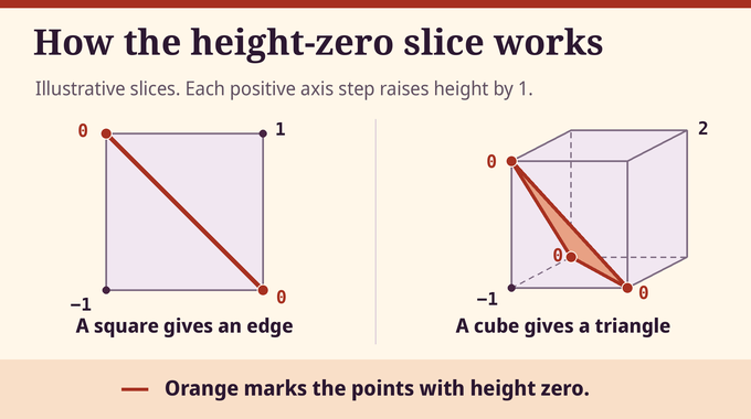
The cubical model for uses a coordinate circle per generator and a coordinate torus per clique. A triangle in gives a three-torus, and there are no larger cliques. The model has a contractible three-dimensional universal cover . Height extends affinely across each cube. The level has vertices indexed by , diagonals of commuting squares, and triangles from slicing three-cubes at coordinate sums one or two.
Triangulating the ambient cubes shows that the links upward and downward at a vertex are subdivisions of . Passing an integer height attaches cones on those links, which preserves homology since the links are acyclic. Each closed height halfspace retracts onto the appropriate subcomplex spanned by vertices, and both halfspaces are acyclic. The Mayer–Vietoris sequence for their union then gives integral acyclicity of their intersection .
The free action on has one vertex orbit and finitely many edge and triangle orbits. Let be the indexed alphabet of oriented edge representatives and the indexed list of triangle words. With , the augmented cellular chain complex is exact.
Here the parenthesized superscripts index direct sums and the augmentation sends group elements to one. The length-two resolution gives . Three commuting directions in a triangle of embed in , and their height-zero subgroup is . Restricting projective modules to that subgroup preserves projectivity. Since its second integral cohomology is nonzero, this forces .
8. Why an Acyclic Two-Dimensional Complex Is Not Enough
Integral acyclicity makes every integral one-cycle a boundary. Simple connectivity asks whether every closed path can be contracted, a question that depends on the order in which edges are traversed. For example, the commutator traverses each based loop once in each direction and has zero edge chain. For unit-quaternion products and on the two loops, the commutator product is . The chain stays zero.
The quotient has as a regular cover with deck group . Its chain complex already computes what the proof needs for cohomological dimension. A two-dimensional classifying space would have a contractible universal cover, and ruling out one cover leaves every other possible presentation to consider. The comparison theorem uses the hypothesized contractible cover to force a property of edge labels on the original graph.
9. The Presentation-Comparison Theorem: How the Obstruction Works
9.1. Matching Triangle Chains to Relator Chains
Exactness and the absence of three-cells make the triangle boundary chains a free basis of . Here is a word in , and its chain records signed edge traversals based at the identity. These words have value one in . A basis of chains by itself gives no description of which words normally generate the relations.
Assume a two-dimensional classifying space exists. Collapse a maximal tree in its one-skeleton to obtain an aspherical presentation. The paper adds defining relators and changes generators and relator words to obtain the original alphabet together with extra letters that represent the identity, so their edges are loops. The new relator list presents . Distinguished relators have exactly the chains , and the other relators project to a free basis in the extra-edge coordinates. The construction allows arbitrary sets of generators and relators.
9.2. Why the Discrepancy Is Quadratic
An actual presentation expresses each triangle word as a finite product of conjugates of relators and their inverses. Independence of the relator boundary chains makes the translated signed counts reduce to one copy of the distinguished relator at the starting vertex. In quaternion products, canceling factors with matching counts requires reordering them and accounting for conjugation. For unit quaternions , swapping neighboring factors costs at most the following amount.
Let bound the distances of the original edge labels from one, and let be the supremum of the distinguished relator products’ distances from one. Once a fixed finite subset of ordinary equations holds, the paper bounds the discrepancy between triangle and distinguished products by for a uniform constant . The quadratic estimate excludes an intermediate value when the original labels are sufficiently small. This keeps solutions with small distinguished products separated from other solutions as the labels vary.
9.3. Solving on Finite Quotients and Returning to the Group
On a finite quotient, take finitely many ordinary relator equations. Their independent exponent rows in the extra loop labels give a nonsingular square minor, so one can select as many quaternion unknowns as equations. Start with all prescribed labels equal to one. Lemma 2.1 gives a nonzero mapping degree in the conjugation-invariant region of small distinguished products. The torus roots contribute with the same sign, and the proof uses conjugation by a cyclic group of sufficiently large prime order so the remaining roots contribute in multiples of that prime. The degree therefore detects a solution inside the specified region. Turning on the prescribed labels preserves this degree because the quadratic estimate keeps roots off its boundary.
Each finite collection of constraints uses only finitely many original edges. Residual finiteness gives a quotient separating their starting vertices, so the needed labels can be copied there and a solution pulled back for those constraints. Compactness of the product of unit quaternion groups yields one assignment satisfying all ordinary equations, with . Write for the bound on the prescribed labels. The quotient may vary with the constraints. When every triangle product equals one, the estimate reduces to with . Hence . All relators now have product one at every vertex. Since they present , every closed path must have trivial product.
10. Constructing Tiny Quaternion Labels With Nontrivial Holonomy
10.1. Turning Reduced Traces Into Directions
A reduced trace remembers the occurrences in a shortest word and their dependency order, identifying words that differ by commuting independent letters. Minimal occurrences have pairwise commuting, distinct directions. Assign each occurrence to the first of its minimal predecessors’ directions in a fixed ordering, then normalize the counts to a barycentric point of . A generator step adds or removes one maximal occurrence. Retained assignments stay fixed, so the two direction vectors lie in a common simplex and differ in ℓ₁ distance by at most if the longer word has length .
Translate the level by , where has height , with . An edge can be traversed via the height-one corner of a commuting square before translation. The translated words are long enough to give image diameters at most for each edge and for each triangle boundary. These bounds concern images in . Continuity will convert them into quaternion labels as small as required.
10.2. Following a Loop One Subdivision at a Time
For an edge with directions , use the height-zero vertices below, where .
The commuting letters give two independent chains in the reduced trace after removing on the left. Their lengths are and . The direction map therefore puts vertex exactly of the way from to . At , the five points occur at . Joining such paths realizes a subdivided copy of any chosen edge loop in .
An equivariant map from the universal cover of into assigns a quaternion to each lifted point. It extends over edges by path connectedness and over triangles by simple connectivity of . Label an edge by the inverse of the quaternion at its lifted start times the quaternion at its lifted end. Compactness of lets sufficiently small images fit inside evenly covered neighborhoods with arbitrarily small variation of the quaternion map on each sheet. Hence individual labels are tiny, and each triangle lifts to a closed loop in one sheet, so its product telescopes to one. A chosen closed path instead lifts from to . If , telescoping yields a conjugate of , which has nontrivial SU(2) holonomy.
11. Completing OpenAI’s Proof: Why Every Two-Dimensional Classifying Space Fails
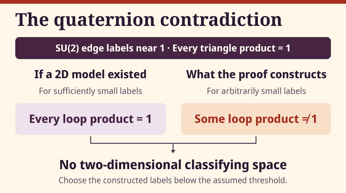
Theorem 3.1 forces trivial holonomy below a positive threshold if a two-dimensional classifying space exists. Proposition 5.1 gives an assignment below any positive threshold with nontrivial holonomy on a closed path. The contradiction excludes every two-dimensional model. The quotient provides a three-dimensional classifying space, giving the claimed geometric dimension.
OpenAI’s accompanying Lean theorem, released with its October mathematics collection, states finite generation, residual finiteness, cohomological dimension two, existence of a three-dimensional classifying space, and exclusion of a two-dimensional one. This Eilenberg–Ganea counterexample settles the original dimension-two question. Whether a finitely presented group exhibits the same gap remains open in the manuscript, and Whitehead’s conjecture is left unresolved. Follow Binary Verse AI for more research explainers in geometric group theory, including the Cannon conjecture and the Boone–Higman conjecture.
Has the Eilenberg–Ganea conjecture been disproved?
Yes. OpenAI’s September 2026 manuscript proves that a finitely generated, residually finite group has integral cohomological dimension two and geometric dimension three. The argument rules out every two-dimensional classifying space for this group, regardless of its number of cells.
How can a group have cohomological dimension two but geometric dimension three?
Cohomological dimension measures the minimum length of a projective resolution of the trivial group-ring module. Geometric dimension measures the minimum dimension of a classifying space with contractible universal cover. The example admits a length-two free resolution and requires at least three dimensions for a classifying space.
Why didn’t the original Bestvina–Brady construction already disprove the conjecture?
Bestvina and Brady showed that at least one of the Eilenberg–Ganea and Whitehead conjectures fails. That result left open the geometric dimension of their candidate groups. OpenAI’s presentation-comparison theorem provides an obstruction that applies to every possible two-dimensional classifying space for its group.
Why isn’t an acyclic two-dimensional complex sufficient?
Acyclicity means that reduced integral homology vanishes. Acyclic complexes can still have nontrivial fundamental groups. A classifying space needs a contractible universal cover, so the proof must exclude every candidate two-dimensional classifying space for the group.
Why does the proof use SU(2) and quaternions?
Unit quaternions give edge labels whose ordered products equal the identity on every triangle but differ from the identity on a particular closed path. For any abelian target, flat labels would give a closed-path product that factors through the first integral homology of the level complex, which vanishes.
Is OpenAI’s Eilenberg–Ganea counterexample finitely presented?
No. The group is finitely generated, residually finite, and of type FL, with a length-two resolution by finitely generated free modules. The seed flag complex has nontrivial fundamental group, which rules out finite presentation by the Bestvina–Brady criterion. The manuscript leaves the finitely presented case open.
Does this proof also resolve Whitehead’s conjecture?
No. The paper settles the Eilenberg–Ganea conjecture by giving an unconditional counterexample. The question of whether every connected subcomplex of an aspherical two-dimensional CW complex is itself aspherical remains unresolved by this proof.