

Give every vertex exactly three neighbors and ask a random walk to forget where it started. Two densely connected regions joined by a handful of edges can trap the walk for a long time, even when every vertex has the same degree. A Ramanujan graph meets the sharp asymptotic spectral standard for avoiding that kind of bottleneck. OpenAI’s September 2026 preprint proves that a deterministic polynomial-time algorithm can build a simple, connected, nonbipartite Ramanujan graph for every fixed degree of at least three and every sufficiently large even number of vertices. Its central move is to build a graph whose spectrum almost fits, then rewire selected edges to move both spectral extremes strictly inside the target interval.
Table of Contents
1. What Is a Ramanujan Graph?
| Feature | Guarantee |
|---|---|
| Allowed degree | Any fixed integer |
| Vertex count | Every sufficiently large even |
| Graph type | Simple, connected and nonbipartite |
| Spectrum on mean-zero vectors | Strictly inside |
| Output and time | Full adjacency list in polynomial bit time for fixed degree |
A graph has vertices and edges. In a -regular graph, every vertex has exactly neighbors. The adjacency matrix of a simple graph has a one where two vertices are adjacent and a zero elsewhere. The all-ones vector is an eigenvector with eigenvalue , since each row sums to . The remaining modes live in , the space of vectors whose coordinates sum to zero.
A connected regular graph is Ramanujan if the absolute values of its nontrivial adjacency eigenvalues are at most . The standard convention sets aside and, for a bipartite graph, . Small nontrivial eigenvalues limit the extent to which large groups of vertices can keep their edges to themselves. This is how a sparse expander graph can have strong global connectivity with a fixed number of edges per vertex.
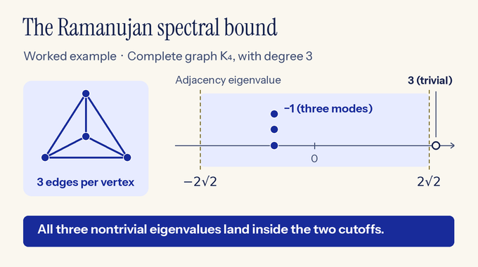
For degree three, the cutoff is . The complete graph on four vertices, , has eigenvalue on constant vectors and on all three remaining modes: its adjacency matrix is the all-ones matrix minus the identity. The largest nonconstant magnitude is therefore , and the top adjacency spectral gap is . The theorem’s challenge is to guarantee strong expansion as the requested order grows.
2. The Spectral Gap and the Alon–Boppana Bound
In spectral graph theory, the adjacency spectral gap of a connected regular graph is , where is the second-largest adjacency eigenvalue. A simple random walk moves to a uniformly chosen neighbor at each step, so its transition matrix is . Every mean-zero mode is multiplied after each step by its eigenvalue divided by . Thus the largest absolute eigenvalue on that subspace controls how fast deviations from uniformity decay in Euclidean norm. Large negative eigenvalues matter because their modes alternate sign and can decay slowly.
The infinite -regular tree supplies the scale. Beyond the root, each vertex has forward branches. After radial levels are normalized by the square root of their size, the adjacency operator between successive levels away from the root has coupling . The tree’s adjacency spectral radius is . The Alon–Boppana bound says that along any fixed-degree family tending to infinite order, the lower limit of the second-largest adjacency eigenvalue is at least that value. The bound concerns growing families, so the four-vertex example can sit well inside the interval.
3. Why Exact Ramanujan Graph Construction Was Difficult
Classical arithmetic constructions attain the tree bound in selected degrees and on particular sequences of graph orders. Morgenstern’s constructions cover degrees one greater than a prime power. Interlacing-polynomial methods reach every degree in the bipartite setting, where flipping the signs of an eigenvector on one side flips the sign of its eigenvalue. In that setting, controlling the upper nontrivial edge controls the lower one by symmetry. A nonbipartite graph requires a separate estimate at each edge.
Earlier deterministic near-Ramanujan algorithms allowed an arbitrarily small fixed positive error. Alon’s construction reached every sufficiently large order for which the degree times the order is even. Random graph results went further: Huang, McKenzie and Yau obtained an asymptotic probability of approximately 69 percent for the exact two-sided event in uniformly random simple regular graphs of fixed degree. Sampling can therefore find examples. A deterministic graph construction has to make reproducible choices and guarantee a passing graph at the specified order. Removing the positive error calls for control of the few eigenvalues closest to the thresholds.
4. OpenAI’s Main Theorem: Every Fixed Degree and Prescribed Even Order
Theorem 1.1 of the manuscript fixes an integer . For each such degree there is a threshold and a deterministic algorithm that, for every even , outputs the full adjacency list of a simple -regular graph on vertices. Every eigenvalue of restricted to satisfies the strict inequalities
The inequality gives two structural consequences. If there were multiple components, one could assign different constants to them to produce a mean-zero eigenvector with eigenvalue . A bipartite regular graph would have a mean-zero vector taking opposite signs on its two sides, with eigenvalue . The strict interval excludes both. The degree-sum formula requires even order for odd degrees. For even degrees, it also permits odd orders, which lie outside this theorem’s guarantee.
5. Inside OpenAI’s Proof: The Four-Stage Construction
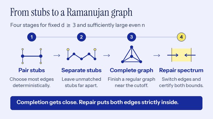
5.1 Deterministic Pairing
Give every vertex one stub for each edge it must ultimately have. Join stubs in pairs, choosing each pair by a score that balances several estimates. The algorithm builds most edges while keeping both spectral edges under control.
5.2 Boundary Separation
Use the next pairings to remove leftover stubs that are clustered or sit near a short return path. The surviving stubs are separated in the partial graph, so their interactions can be estimated during completion.
5.3 Graph Completion
Join the remaining stubs using estimates of how each added edge changes the inverse matrices. The result is a regular graph with a very small possible spectral excess and enough information about its eigenvectors to guide the repair.
5.4 Exact Spectral Repair
Select disjoint edge switches that preserve every vertex’s degree. Choose the switches so they give the weakest spectral modes at both ends an inward push, then test both strict inequalities exactly.
OpenAI attributes the release to an internal frontier model. This preprint is family 178. The public collection contains process summaries for selected problems, with no discovery trace for this construction. The roadmap follows the manuscript’s proof structure.
6. Deterministic Pairing Through Discounted Statistical Accounts
A uniform pairing of the stubs is the usual configuration model. The proof uses its averages for derandomization by conditional expectations. A single choice must maintain local structural counts, matrix traces and bounds on individual inverse entries. A move that helps one statistic may hurt another.
Lemma 3.1 gives each nonnegative statistic, or account, a separate discount. At each step the algorithm divides that discount by the larger of one and the ratio of the account’s conditional expected next value to its current value. With the updated discounts, the average total across candidate moves is at most the current total. The algorithm takes a minimizing move. Bounds on how the discounts accumulate let the proof recover bounds on the original statistics. High even moments help convert the aggregate control into a maximum bound over polynomially many entries.
The main analytic objects are signed precision matrices, which at completion become on the mean-zero subspace, with the identity, and above the tree threshold. Positivity for the two signs tests the two spectral edges. The proof compares normalized inverse entries with weighted sums over nonbacktracking paths, which may revisit vertices but may never reverse the edge just taken. These comparisons supply the estimates that cleanup must preserve.
7. Separating the Unresolved Boundary
At the next stop, each remaining stub must sit at its own vertex. There must be no short nonempty nonbacktracking path joining two such vertices or returning to the same one. The cleanup pairs the initially problematic stubs first, choosing eligible partners from the initially clean set. Prescribing one endpoint changes the conditional averages, so the proof bounds the accumulated effects of these choices through path sums along the selected history.
Separation prevents a new edge from interacting with another unresolved vertex through a short route made of old edges. It also makes every perfect matching of the remaining stubs graph-theoretically admissible: each added edge is simple and preserves the construction’s short-cycle exclusion. The remaining question is which matching preserves the spectral estimates.
8. Completing a Near-Ramanujan Graph
The proof freezes a smoothly truncated path sum at the separation stop. Its restriction to boundary contrasts, combinations of unresolved-stub coordinates that sum to zero, is close to the identity on that subspace. For each vertex row, at most one boundary coordinate is substantial. The Woodbury identity computes the inverse change from each low-rank pairing update, so the same reference can be continued as the boundary shrinks.
The algorithm first reduces squared row energies, which measure the compressed inverse’s deviation from the identity on the unresolved contrasts. Those smaller energies then help bound the fluctuations of individual entries. With these bounds in place, even an arbitrary matching of the last few stubs fits the estimates. The completed graph’s nonconstant eigenvalues obey
The reference still varies smoothly with the spectral parameter. Its diagonal behavior and the retained path data supply the two local estimates used in the final stage.
9. Exact Spectral Repair Through Biased Edge Switches
9.1 Isolating the Modes That Need Repair
Write and let be the signed slack of a nonconstant eigenvalue . Negative slack means that eigenvalue is outside the target at sign . Lemma 8.1 bounds the combined squared amplitude at any one vertex of the orthonormal modes within slack of an edge by a constant times , for . Summing over vertices bounds the number of modes needing repair. Their small local mass also limits how much a switch can perturb the near-edge subspace.
Choose a cutoff for each sign and call the modes farther from the edge the bulk. The bulk resolvent weights those modes by the reciprocals of their positive slacks. For most edges, the two-by-two block on the endpoints is close to the corresponding infinite-tree block. Theorem 8.3 uses this estimate to show that the updated bulk remains positive and to eliminate it by a Schur complement. In effect, the calculation folds the bulk’s response to rewiring into a smaller matrix on the near-edge modes. Positivity of that smaller matrix finishes the test at the relevant edge.
9.2 Giving Both Spectral Edges an Inward Shift
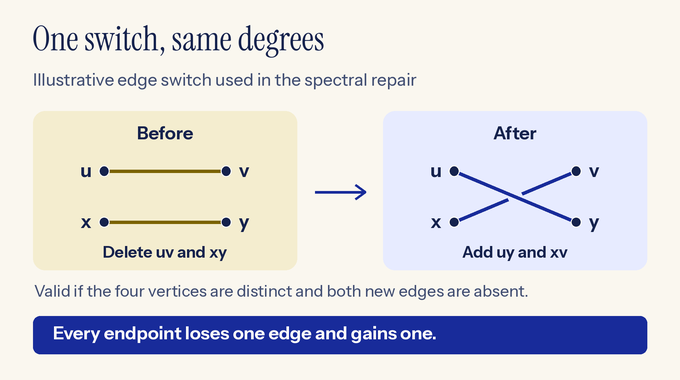
A valid switch deletes the edges and , then adds and . Four distinct endpoints and absent replacement edges preserve simplicity, while each endpoint loses and gains one neighbor. Under uniform edge-pair sampling, the mean idealized correction per switch for mode is . Over the chosen number of switches this just rescales each slack by a positive factor, preserving its sign.
The paper tilts the joint distribution of the two edges using the eigenmodes closest to either threshold. Both edges still have uniform marginals before conditioning on typical edges. What changes is how their endpoint amplitudes are correlated. The cross-edge terms then contribute a positive mean correction that exceeds the possible spectral excess for those modes. The other near-edge modes keep a fixed fraction of their existing slack. Local mass and the endpoint block estimates make the errors smaller than the available margin. One collection of valid, vertex-disjoint switches therefore makes both signed precisions at strictly positive on the mean-zero subspace.
10. Algorithmic Complexity and Exact Verification
The distribution in the repair proof establishes that successful switches exist. The algorithm finds them deterministically by enumerating a polynomial-size family generated from pairwise-independent draws. It discards invalid switch collections and evaluates the rest by exact rational arithmetic. If has columns forming a rational basis of and is the candidate’s adjacency matrix, the acceptance test is
The symbol means positive definite. On an eigenvector of in the tested subspace, the middle matrix acts by . Rational elimination thus certifies both strict bounds without rounding the eigenvalues. The theorem gives bit operations for a degree-dependent exponent . That is an asymptotic guarantee for producing the full adjacency list. The manuscript gives no benchmark for practical graph sizes and no local adjacency-query bound.
11. OpenAI’s Proof Versus Previous Ramanujan Graph Constructions
| Approach | Degree and Order | Spectrum and Graph Type | Algorithmic Guarantee |
|---|---|---|---|
| Arithmetic families | Restricted degrees; arithmetic sequences of orders | Exact; nonbipartite families available | Explicit arithmetic constructions |
| Bipartite interlacing | All degrees; simple at multiples of ; multigraphs at every even order | Exact after excluding ; bipartite | Deterministic polynomial time for the matching multigraph construction (Cohen) |
| Deterministic near-Ramanujan | All fixed degrees; every sufficiently large order with even (Alon) | Tree bound plus fixed positive error; simple and nonbipartite for sufficiently small error | Deterministic polynomial time |
| Random regular graphs | All fixed degrees; large orders with even | Exact with limiting probability about 69%; simple, with both spectral edges tested | Random existence via edge universality |
| OpenAI preprint | All fixed degrees; every sufficiently large even order | Strictly inside both tree edges; simple and nonbipartite | Deterministic polynomial bit time; full adjacency list |
The main advance is the combination of exact two-sided control, simplicity, nonbipartiteness and prescribed orders in one deterministic algorithm. In the bipartite literature, the closest order guarantee at the exact threshold applies to multigraphs. In the deterministic near-Ramanujan literature, the closest order guarantee for simple graphs still includes a positive spectral allowance.
12. What the Result Changes and What Remains Unsolved
The theorem gives theoretical computer science a way to specify a network’s even vertex count and fixed degree in advance and obtain a graph with the full Ramanujan guarantee. In sparse communication networks, this mathematical guarantee concerns connectivity and the decay of random-walk modes. Practical construction times and usable size thresholds remain to be established.
The Bilu–Linial conjecture asks for a two-lift of an arbitrary regular input graph whose new eigenvalues satisfy the two-sided tree bound. This construction starts from empty stubs and builds its own graph, leaving the signing problem open. The public manuscript directory provides a preprint, with no accompanying Lean formalization listed. The exact acceptance test verifies the spectrum of an individual candidate, while the manuscript’s argument explains why the search must find one.
The Ramanujan graph construction shows what extra information can buy at a sharp spectral threshold: local eigenvector and resolvent estimates make it possible to repair both edges with degree-preserving switches. Follow Binary Verse AI for more research explainers on graph algorithms and AI-generated mathematics.
What is a Ramanujan graph?
A Ramanujan graph is a connected regular graph whose nontrivial adjacency eigenvalues have absolute values at most twice the square root of one less than the vertex degree. The degree eigenvalue is trivial, and its negative is also trivial in the bipartite case. The bound is asymptotically optimal for fixed-degree expansion.
Why are Ramanujan graphs important?
They combine sparse connectivity with strong spectral expansion. This makes them useful in theoretical computer science, including pseudorandomness and error-correcting codes, and gives mathematical guarantees relevant to sparse communication networks.
What did OpenAI prove about Ramanujan graphs?
The manuscript gives a deterministic polynomial-time construction of simple, connected, nonbipartite Ramanujan graphs for every fixed degree of at least three and every sufficiently large even vertex count. Every adjacency eigenvalue on the mean-zero subspace lies strictly inside the two Ramanujan bounds.
What is the difference between a Ramanujan graph and an expander graph?
An expander graph combines sparse edges with strong connectivity across cuts. Ramanujan graphs are a special class of spectral expanders that satisfy the sharp asymptotic adjacency bound given by the infinite regular tree.
Why are nonbipartite Ramanujan graphs difficult to construct?
The spectrum of a bipartite graph is symmetric about zero, so an upper bound on the nontrivial eigenvalues also controls the negative edge. Nonbipartite graphs lack that symmetry and require control of both edges.
Can OpenAI’s algorithm generate Ramanujan graphs efficiently?
The manuscript proves polynomial bit complexity when the degree is fixed. The polynomial exponent and minimum covered graph order can depend on the degree. Practical runtime and scalability remain unmeasured in the paper.
Does OpenAI’s proof solve the Bilu–Linial conjecture?
No. The conjecture asks for a two-lift of an arbitrary regular input graph with all new eigenvalues within the two Ramanujan bounds. OpenAI’s algorithm constructs a new graph through stub pairings and degree-preserving edge switches.