
Why are ellipses special billiard tables? Send a ball around an elliptical table at a shallow angle and every leg of its path can stay tangent to the same invisible inner ellipse. The Birkhoff conjecture asks whether that kind of order forces the table itself to be elliptical. OpenAI’s September 24, 2026 manuscript proves the near-boundary version: a smooth, strictly convex planar table of positive curvature must be an ellipse if a full band inside its boundary is continuously filled by smooth convex billiard caustics. The proof extracts analyticity from the band, then shows that any surviving nonelliptical shape would require a complex continuation that contradicts its own reflection equations.
Table of Contents
1. What Is the Birkhoff Conjecture?
In mathematical billiards, a point moves along straight segments inside a domain and reflects elastically at the wall. The billiard map records one collision after another. Integrability here means an invariant family that organizes the motion. A trajectory in that family stays on the same invariant curve in the space of oriented lines. In the table itself, the associated caustic is an envelope of those lines. The unrelated Pierce–Birkhoff conjecture concerns representations of piecewise polynomial functions.
| Question | What the Manuscript Establishes |
|---|---|
| Which tables? | Bounded, smooth, strictly convex planar tables with positive curvature everywhere. |
| Which invariant data? | A full collar of smooth closed convex caustics, continuously parametrized up to the boundary. |
| What follows? | The whole boundary is elliptical. A circle counts as an ellipse. |
| Which tools? | Rational action constraints, complex continuation and a stopped Brownian argument. |
A single periodic polygon imposes an equal-angle condition at its vertices. A full collar demands compatible reflections at every starting location across an interval of grazing directions.
2. Why Are Elliptical Billiards Special?
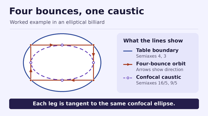
At a collision, the component of velocity along the wall is preserved and the normal component reverses. In an ellipse this law preserves tangency to a member of a confocal family. For outer semiaxes and , with , the inner confocal ellipses have squared semiaxes and for . Their common squared focal distance is . As tends to zero, these caustics approach the table boundary and fill a collar.
Take an ellipse with semiaxes 4 and 3 and a horizontal trajectory along , moving right. Its first impact on the right is . The normal is proportional to , so the ball turns straight down. By symmetry it traces a rectangle, whose four sides touch the inner ellipse with semiaxes and . Both ellipses have squared focal distance 7.
3. Why the Birkhoff Conjecture Was So Difficult to Prove
Lazutkin’s theorem gives a positive-measure family of grazing caustics for sufficiently smooth, positively curved boundaries, with gaps between the invariant curves. The Marvizi–Melrose construction gives an interpolating integral with an error flat at grazing, meaning the error vanishes to all orders there. The new proof needs exact action identities from invariant leaves.
| Result | Hypotheses and Reach |
|---|---|
| Lazutkin (1973) | Produces a positive-measure grazing family for sufficiently smooth, positively curved tables. The family leaves gaps. |
| Marvizi–Melrose (1982) | Obtains an asymptotic grazing integral with an error flat at the boundary. |
| Kaloshin and Sorrentino (2018) | Proves rigidity for sufficiently small integrable perturbations of an ellipse. |
| Bialy and Mironov (2022) | Uses central symmetry and a foliation reaching rotation 1/4. The physical caustic version assumes a continuously differentiable foliation. |
| OpenAI (2026) | Proves ellipse rigidity from a full continuous physical collar of smooth convex caustics in the positively curved smooth class. |
Perturbative rigidity starts with a known ellipse and controls the permitted deformations. Here the initial table can be far from every ellipse. Even the analyticity needed to use complex singularities has to be earned from the real billiard dynamics.
4. What OpenAI’s Birkhoff Conjecture Proof Establishes
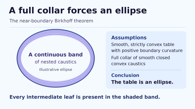
Definition 1.1 assumes a bounded strictly convex domain whose boundary is a smooth, regular simple closed curve with everywhere positive curvature. Every interior leaf is itself a smooth, regular simple closed curve bounding a strictly convex set. Its tangent billiard segments remain tangent after reflection at either endpoint. A homeomorphism from a circle times the half-open interval fills a relatively open neighborhood in the closed table, with the boundary at parameter zero. This gives continuity across the leaves and smoothness along each one.
Theorem 1.2 says that the domain is an ellipse, with circles included. Here is its center, is a planar point, is a real symmetric positive-definite matrix, and the superscript denotes transpose.
OpenAI attributes the release’s results to an internal frontier model. The repository lists reasoning summaries for selected families. Family 147, the near-boundary Birkhoff conjecture, is absent from that list and from the public Lean catalogue. The roadmap follows the dependencies of the written proof.
4.1. The Proof in Five Stages
- Turn nested caustics into periodic families. On a suitable rational leaf every starting point closes after the same number of reflections, giving exact constraints on the table’s shape.
- Recover analytic coordinates. Use the periodic constraints first to upgrade the wall’s regularity and then to make the near-grazing dynamics analytic in both phase and leaf parameter.
- Continue the reflections into the complex plane. Finite chains tie their interior to their endpoints. A special type of complex tangency already forces an ellipse.
- Classify the other continuations by growth. Quiet regions would let the proof cross an impassable boundary. Rescalings of excessively fast growth also lead to contradictions, leaving one critical case.
- Test a fixed odd periodic chain in that critical case. Track its coupled impacts along stopped Brownian paths. The last impact to cross a selected row cannot move far enough to reach the depth that the continuation requires.
5. How Rational Caustics Force Analytic Regularity
The rotation number measures average turns per reflection. Nesting strictly orders the induced maps on oriented tangent lines. An interval of leaves sharing a rational rotation would contradict that ordering: preservation of area makes almost every point recurrent, but between fixed points of a lifted return map motion is monotone. Each sufficiently small positive rational rotation thus has a unique leaf. Comparing it with the leaves on either side shows that every point on it is periodic. At rotation , for example, the orbit makes one turn in reflections.
Write for the support function, the distance to the supporting line measured along the unit outward normal at angle , with the origin in the interior. The curvature radius is , where primes denote angle derivatives here. A grazing coordinate absorbs the leading curvature dependence. The normalized generating action differs from the original reflection action by a change of coordinates, a scaling, and a term that telescopes. Its stationary polygon equations still encode reflection.
The action is constant along each periodic family because every polygon in the family is stationary, including the endpoint variation around the closed cycle. A constant action has zero nonzero Fourier modes. The proof extracts the constraint at index from the corresponding stationary action. The high-frequency system has a derivative close to the identity. Holding the low modes fixed, a Newton construction in an exponentially weighted Fourier space, followed by uniqueness among smooth solutions, identifies the actual boundary with a real-analytic one.
6. Constructing a Jointly Analytic Billiard Collar
An analytic boundary still leaves a question about the dependence of the orbits on the leaf. The paper seeks a phase coordinate in which reflection is translation by , the angular rotation increment. At grazing, . In a Fourier mode, the centered difference for this translation carries a sine factor that vanishes at rational resonances. Division at such points is the obstacle to constructing a joint analytic solution.
Actual periodic leaves supply both the value and first-parameter compatibility required for two successive divisions. The first parameter jet is constructed using rational periodic meshes and the normalized equation. It is a derivative of the constructed correction. Successive Newton steps then produce a change of coordinates even in , with furnishing analytic coordinates on the phase collar. In these coordinates is a first integral. Joint analyticity lets the next stage vary both phase and parameter over complex values.
7. Complex Continuation and the Geometry of Reflected Chains
The continued billiard replaces a real path by a chain of projective lines and their impact points. At a regular impact the complex reflection law is still rational in the incident line and tangent. The issue is whether analytic continuation around a singularity could return a different branch, even when part of a chain is already known.
Using finite systems for endpoint derivatives and a scaling in which impacts coalesce at grazing, the manuscript derives algebraic constraints on intermediate lines or impacts from endpoint jets. If a patch existed at a first finite continuation wall, those constraints would control possible branch changes. The even dependence on and product continuation make the patch incompatible with maximal strip width. The boundary curve inherits the same no-patch property at its finite first wall.
8. The Shape Coordinate and the Ellipse Rigidity Mechanism
The normal angle is encoded by . Its meromorphic extension can have a zero or a pole at an isotropic tangency, where a nonzero complex tangent can have zero squared length for the bilinear Euclidean product. Such a center gives a local reflection symmetry of the complex boundary. The symmetry would cross any finite strip edge. With an infinite strip, conjugate centers give a second period, making the normal a doubly periodic meromorphic function.
The centers constrain the degree of this function to two and lead to an even quartic equation for the square of its derivative as a function of the normal. On the real curve this forces the square of the normal-angle derivative to be a positive quadratic form in the unit normal direction. The resulting curvature radius is that of an ellipse. A support function is determined by its curvature radius up to translation, so the boundary must be elliptical.
When the normal has neither zeros nor poles and the table is not a circle, the proof instead lifts every continued impact to one intrinsic coordinate in the boundary’s shape strip. This lift is single-valued even where the affine impact coordinates have poles.
9. Eliminating Impossible Growth Profiles
Let be the shape strip’s half-width, the derivative of the normal angle in , and its associated second-derivative quotient. In this part denotes a field, rather than a period denominator. Both fields are holomorphic in the nonisotropic case. The growth quantity is
The normalized chord action compares arc and chord lengths. Expressing them through kernels of second-order differential equations makes apparent divisions by zero removable in the relevant small-field regime. The resulting recurrence is close to one with equally spaced impacts. This allows continuation through complex cones wherever the rescaled fields stay small. A quiet profile even at an individual center can provide a patch and so break the first-wall constraint.
At larger growth scales the argument takes limits of the rescaled fields and tracks the corresponding impact equation. Finite superlinear growth violates the continuation and shape-strip constraints. Exponential profiles produce a model with nontrivial branching that the single-valued lift cannot realize. These exclusions leave a finite wall where the upper growth order of in inverse distance to the edge is exactly one.
10. Critical Moment Estimates and the Angle Budget
Pointwise control at the critical scale permits large spikes. The proof instead measures the fields across horizontal rows and groups neighborhoods by distance to the wall. With depth , the first-field moment is the horizontal root-mean-square of . A bootstrap improves row bounds, conditional on ruling out a specific sequence of extreme profiles.
The limiting moment law splits that exclusion into two cases. Steep growth gives an exponential profile already ruled out. The other case isolates a nonzero limiting first field. The proof tracks where that field has large modulus, routing paths through those regions across multiple scales. A contradiction between the required high-value witnesses and the allowed growth rules out the limiting field. Only then does the conditional estimate become an angle budget. For sufficiently large logarithmic depth , the integral of the squared first-field moment satisfies the bound below, with a constant , a fixed starting depth level and exponent . The power saving over quadratic growth controls the angular variation available to the periodic impacts.
11. How Brownian Motion Completes the Rigidity Proof
Take a fixed odd number of impacts at angular step . Oddness eliminates the alternating mode, so the impact normals uniquely determine the edge angles. The cyclic Jacobi matrix, a second variation of polygon length in adapted coordinates, relates the derivatives of neighboring impacts. Appropriate reduced matrices are invertible on the real slice, giving determinants whose size can be controlled probabilistically after continuation.
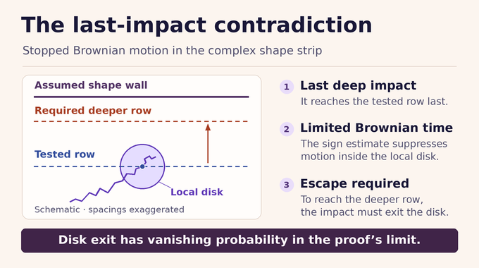
The proof runs planar Brownian motion in the complex phase strip, stopping by the deepest shape-strip level visited so far. Each holomorphic impact coordinate maps this motion to a Brownian path with its own clock. Occupation estimates control the clocks, while the angle budget bounds the accumulated quadratic variation of the normal angles. These estimates constrain the reflected-chain geometry even as some impacts approach the wall. A deterministic row can then be selected where is strongly positive or strongly negative almost everywhere and keeps that sign in small disks around typical crossing points.
The matrix identities suppress the last deep impact’s motion in either sign case. At its first crossing of the chosen row, its probability of landing in a suitable disk tends to one. Its remaining clock makes leaving the disk overwhelmingly unlikely, yet it must leave to reach its prescribed deeper level. That contradiction rules out the critical wall and completes the classification.
12. What the Proof Means for Billiard Dynamics
The near-boundary Birkhoff conjecture now has a proof in the stated smooth, positively curved class. The implication reaches the entire shape of the boundary from trajectories in an arbitrarily thin filled collar. Lower boundary regularity calls for a separate argument, and a family with gaps is compatible with nonelliptical tables. The finite-chain determination argument and the transfer from complex growth bounds to stopped motion offer concrete methods for related rigidity questions.
Follow Binary Verse AI for more paper-led explainers on dynamical systems, including irrational triangular billiards, the standard map and Shub’s entropy conjecture, and explore our coverage of AI-generated mathematical proofs.
What is the Birkhoff conjecture?
The Birkhoff conjecture asks whether every sufficiently smooth, convex, integrable planar billiard table must be an ellipse. It concerns the relationship between the geometry of the wall and the dynamics of reflected trajectories.
Has OpenAI solved the Birkhoff conjecture?
OpenAI’s September 24, 2026 manuscript proves the near-boundary Birkhoff conjecture for smooth, strictly convex planar billiards with positive curvature and a continuous collar of smooth closed convex caustics. The theorem applies under these specific hypotheses.
Why are elliptical billiards integrable?
Elliptical billiards have confocal conics that act as invariant caustics. A trajectory tangent to one of these caustics remains tangent after successive reflections, so the same caustic organizes its entire orbit.
What is a continuous caustic collar?
A continuous caustic collar is a full neighborhood inside the billiard boundary filled by a continuous family of nested, smooth closed convex caustics. Every intermediate leaf is present, so the collar has no gaps.
How does OpenAI’s proof differ from previous Birkhoff conjecture results?
Earlier results established rigidity near an ellipse, under central symmetry with specified foliation conditions, or under other stronger hypotheses. In OpenAI’s theorem, the starting table can be any smooth, strictly convex table of positive curvature with a continuous caustic collar. The proof derives real analyticity from the filled collar.
Why does the Birkhoff conjecture proof use Brownian motion?
Brownian motion samples the complex phase of a fixed odd periodic chain. Stopped paths and occupation estimates control how the chain’s impacts can move near a potential continuation boundary. A sign test shows that the last deep impact is overwhelmingly unlikely to move as far as the continuation requires, ruling out the remaining case.