
An edge in a segmented image can run through a region, stop inside it, or meet two other edges. Could an energy minimizer hide a disconnected crack among other cracks, even as you zoom in? The planar Mumford Shah conjecture asks whether those three patterns describe every interior point of the discontinuity set. OpenAI’s September 24, 2026 manuscript proves that they do for reduced absolute minimizers with bounded fidelity data. The proof closes a gap in the classification of blow-up limits by ruling out bounded connected crack components when the complement of the limiting crack is connected.
Table of Contents
1. What Is the Mumford–Shah Conjecture, and What Did OpenAI Prove?
In their 1989 paper on image segmentation, David Mumford and Jayant Shah sought a reconstruction that varies smoothly within regions and can jump across edges. The regularity question asks whether minimizing that energy makes the edges themselves orderly. “Crack” is the mathematical term used here for the closed set where jumps are permitted.
| Aspect | Result |
|---|---|
| Setting | A bounded planar Lipschitz domain with bounded real-valued fidelity data |
| Minimizers | Reduced absolute minimizers under compact interior changes |
| Interior geometry | A regular arc, a crack tip, or three arcs meeting at 120° |
| Key proof step | Exclude isolated compact pieces in blow-up limits with connected complement |
| Component count | Finitely many global crack components meet any relatively compact interior open set |
The result combines an exclusion argument for whole-plane limits with local regularity theorems for the original image model. It also controls the number of global crack components that can enter a region strictly inside the domain. The September manuscript specifies the hypotheses and proof. OpenAI’s October 6 release announcement describes the broader collection in which the work appeared.
2. The Mumford–Shah Functional and the Cost of a Crack
Let be a bounded Lipschitz domain in the plane, the bounded real-valued input, the reconstruction, and its relatively closed crack set of finite length. Equation (1.1) gives the energy on an open subregion .
The first term is the Dirichlet energy, which penalizes gradients off the crack. The second charges its length, measured by one-dimensional Hausdorff measure . The last charges squared error against the data. The pair must have square-integrable on the domain and a square-integrable weak gradient off . Absolute minimality compares simultaneous changes to and supported in a compact subset of an interior comparison region. Reducedness means every sufficiently small disk centered on contains positive crack length.
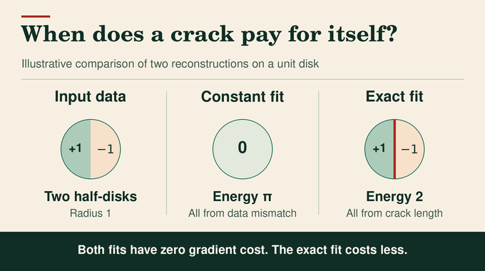
Take a unit disk with input values on the two halves. Reconstructing it by a single constant gives the lowest constant-fit energy at zero, with fidelity cost and zero gradient or crack cost. Reproducing the two values exactly with a diameter as the crack costs in length, with zero fidelity and gradient costs. This comparison of two candidates shows when a jump can pay for itself. It leaves the minimization problem open for that example.
3. The Main Theorem on Regular Arcs, Crack Tips, and 120° Junctions
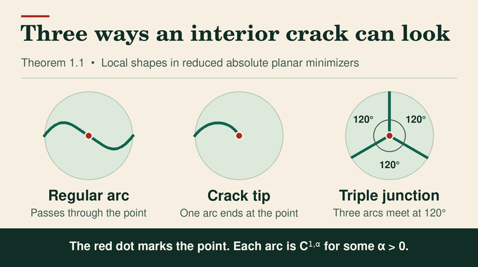
Theorem 1.1 applies to every reduced absolute minimizer under the assumptions above. Each point of has a neighborhood where the whole crack set is a single embedded arc passing through the point, a single embedded arc ending there, or three embedded arcs meeting only there and forming pairwise angles of 120°. The arcs are for some . This means they admit continuously differentiable parametrizations with Hölder-continuous first derivatives. A curved crack can satisfy the theorem. At a junction the angles describe its three outgoing tangents. Equal length weights give the three tangents equal weight in the equilibrium condition.
The theorem also gives finiteness on any open set , meaning that the closure of is compact and contained in . If is the collection of global connected components, the claim takes the following form.
The count tracks components of the original closed crack set. For example, a single line that crosses several disjoint observation windows still contributes one global component.
4. Why Earlier Regularity Results Left a Crucial Obstruction
Bonnet’s blow-up theory classified global minimizers with a connected crack set. Bonnet and David established global minimality of the crack tip, and earlier classification also covered a crack with all but at most one component contained in a common compact set. David and Léger treated global cracks that disconnect the plane. The two connectivity questions are different. A half-line is connected and its complement is also connected. A full line is connected and its complement has two components.
In the generalized blow-up setting, the unresolved case allowed a bounded component when the complement was connected. Separate bounded components might accumulate, making it impossible to move any one of them without disturbing its neighbors. Francesco Deangelis posted a separate proof on September 22, 2026. It uses second variations, a planar Hodge identity and holomorphic rigidity. OpenAI’s manuscript uses finite translations and a harmonic interaction in the translation parameter. In his revised preprint, Deangelis credits ChatGPT Astra with generating the initial proof strategy and draft and takes responsibility for the paper’s mathematics.
5. Proof Stage 1: From Arbitrary Discontinuities to Rectifiable Minimizers
The original admissibility conditions allow any relatively closed set of finite length, so Proposition 2.1 first establishes the structure needed by the classical theory. For almost every interior disk radius, its boundary meets the crack at finitely many points, and the reconstruction has a bounded trace on the remaining arcs. Clip inside such a disk at levels beyond both the trace bound and the data bound. The crack is unchanged, the gradient cost cannot increase, and the fidelity cost strictly falls wherever clipping takes effect. This yields local boundedness.
Covering the crack by small disks with controlled total perimeter then gives locally bounded variation. Off the crack the derivative is absolutely continuous, and the Cantor part, the diffuse singular part of the derivative, gives no mass to a set of finite length. Thus is locally in SBV, the space of special functions of bounded variation. Its approximate jump set is countably rectifiable, with two distinct one-sided approximate limits at jump points. Dirichlet replacements with smoothed boundary traces show that any portion of outside has zero length. Reducedness then identifies with the relative closure of .
6. Proof Stage 2: Blow-Up Limits Reveal the Possible Crack Geometry
Center a microscope at and take a sequence of radii . Proposition 3.1 rescales positions by the radius and function values by its square root.
The gradient energy in two dimensions and the crack length then scale by the same factor. On each fixed rescaled ball, the fidelity cost, divided by the radius, tends to zero because the original function and data are locally bounded. After passing to a subsequence, the rescaled sets converge locally in bilateral Hausdorff distance, which requires each set to lie near the other. The limiting crack contains the origin.
The limiting function is normalized by subtracting a reference value on each component of the complement. The generalized limit also records differences between those reference values, which can diverge. If the complement is connected, there are no distinct exterior components whose separation a competitor must preserve. The limit is then an absolute minimizer for the zero-fidelity energy, the sum of gradient energy and crack length, under compact changes that can meet .
7. Proof Stage 3: Isolating a Compact Crack Island
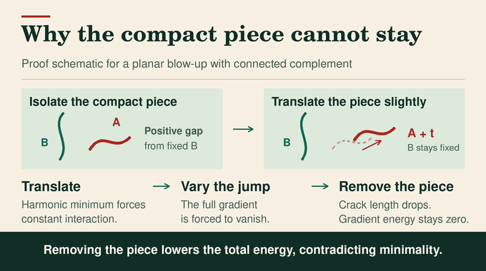
Suppose the limiting crack has a bounded connected component. That component is compact, but adjacent components could approach it arbitrarily closely. Lemma 4.1 encloses it in a larger compact piece at positive distance from the closed remainder . The construction works in the intersection of the crack with a large closed disk. The component can be separated from each point of the crack on the boundary circle by a neighborhood that is both open and closed relative to that intersection. Compactness of the circle portion reduces the construction to finitely many such separations.
The resulting piece can include several components. It has finite positive length because it is bounded, relatively open in the crack, and contains a point in the support of the crack-length measure. Almost every point of the limiting crack by length has a neighborhood containing a single regular arc, so the piece contains one. The gap to gives room to translate by any sufficiently small vector. The complement of remains connected because it contains the original connected, dense complement.
8. Proof Stage 4: Splitting the Gradient Into Two Fields
Choose a smooth cutoff equal to one near and supported away from . Then carries the values of near the compact piece and vanishes far away. Lemma 5.2 projects the gradient density of onto the closed subspace of square-integrable fields generated by gradients of smooth, compactly supported functions. Write for this gradient projection and choose the potential to tend to zero at infinity. This gives a split into two functions.
Here is divergence-free on the whole plane and its distributional curl is supported on . The function carries the possible jump across . It decays like at infinity, and its gradient like . Smooth value variations of give zero distributional divergence for its gradient density. Subtracting therefore gives a divergence-free field . The function extends across , where it equals locally, and is harmonic on the connected complement of . This allows the compact jump to move while stays fixed.
9. Proof Stage 5: How Translation Makes the Harmonic Interaction Constant
Translate to and carry with it while holding and fixed. Write for the translated gradient and for its interaction with . Also allow an independent projected jump perturbation with gradient and real amplitude . Write for its interaction and use the square-integrable vector-field inner product and norm below. The resulting comparison is equation (5.3).
Here translation preserves the crack length and the square norm of . A cutoff on a distant annulus returns the trial function to outside a large disk. The annular error tends to zero because the translated fields decay while the original gradient energy in a radius- disk grows at most linearly in . This makes the energy comparison legitimate even when the total Dirichlet energy on the plane is infinite.
The translation Laplacian of is the rotated gradient of its curl, which is supported on the translated piece. Pairing it near that piece with the curl-free gradient gives zero. Away from the piece the field is harmonic, with decay allowing differentiation of the tail integral. Thus is harmonic in . With , the inequality makes the origin a minimum. The harmonic minimum principle forces to be constant for small translations.
10. Proof Stage 6: How Jump Variations Produce the Contradiction
Once the translation term is constant, (5.3) is a nonnegative quadratic in with zero constant term. Testing amplitudes of both signs makes its linear coefficient vanish. The resulting identity holds for every allowed jump perturbation. The projected potential can be dropped from this pairing by testing the divergence-free equation for with a cutoff. Its decay makes the cutoff error tend to zero.
Along a regular subarc of , vary the trace on one side by an arbitrary smooth function supported inside the arc and keep the other trace fixed. Integration by parts pairs that jump with the normal derivative of on the translated arc. Since the pairing stays constant for every jump test, the normal derivative at any fixed arc point stays constant as that point translates within a small disk. In two dimensions, a harmonic function with a constant derivative in one fixed direction is affine on that disk. Unique continuation extends that conclusion throughout the connected complement of .
A nonzero constant gradient would have quadratic energy growth in the disk radius. The linear bound forces to vanish. Taking the original compact field as the perturbation then forces to vanish as well. With constant on the connected complement of , removing preserves Dirichlet energy and saves its positive length. That contradicts minimality.
11. How Global Classification Becomes Interior Regularity
Corollary 6.1 brings the cases together. If the crack disconnects the plane, the established classification gives a line or a 120° triod, meaning three rays from a common point. If the complement is connected, the compact-piece argument excludes every bounded component. The earlier theory allows at most one unbounded component, so the crack is empty or connected and the existing classification applies. A blow-up at a point of the original crack contains the origin, leaving a line, half-line, or triod.
De Lellis and Focardi’s epsilon-regularity theorem converts geometric closeness to one of those models in a larger disk into a description of the entire crack in a smaller disk. Hausdorff convergence provides the required closeness at some sufficiently small scale. The center of the disk can lie on an ordinary branch even if the model chart contains a nearby tip or junction. Shrinking the neighborhood around the point in question yields the appropriate geometry there. Finally, finitely many connected model neighborhoods cover the compact intersection of with the closure of . Each meets only one global component.
12. The Scope of the Mumford–Shah Interior Regularity Proof
Corollary 6.3 bounds the area where the gradient exceeds a positive threshold . Here denotes planar area and depends on the region and minimizer.
It gives local integrability for . To see the endpoint exponent, consider the crack-tip profile in polar coordinates . Its gradient has magnitude , so for large thresholds the radius of the superlevel disk scales as and the area as . The fourth power of the gradient integrates radially like , which diverges at the tip. Ordinary is therefore too strong as a general conclusion.
The theorem is about the planar interior. Boundary behavior, finiteness up to the boundary, and regularity in higher dimensions lie outside its scope. The released Lean source addresses compact-piece exclusion under its own hypotheses. The full bounded-domain theorem in the manuscript additionally uses the rectifiability, compactness, classification, and epsilon-regularity steps. For segmentation, the result certifies the local geometry of exact minimizers of the continuum energy. A numerical algorithm’s accuracy and runtime require separate evidence.
The Mumford–Shah conjecture comes down to what happens when a hypothetical compact piece has room to move and its jump values can vary. The answer leaves it with no gradient energy to justify its length. Follow Binary Verse AI for more research explainers on free boundary problems, PDE regularity, and Lean formalization.
Has the Mumford–Shah conjecture been proved?
Yes. The planar interior regularity assertion has been proved for reduced absolute minimizers with bounded fidelity data. OpenAI’s September 2026 manuscript also proves local finiteness of global crack components. Boundary regularity and higher dimensions lie outside the theorem’s scope.
What are the three possible configurations of Mumford–Shah minimizers?
Near an interior point of the closed discontinuity set, there is a regular arc passing through the point, a single arc ending there, or three arcs meeting there at pairwise angles of 120°. Each arc is C1,α for some α > 0.
What was the main mathematical difficulty in proving the conjecture?
Earlier classification results left open the possibility of bounded connected crack components in generalized blow-up limits whose complements were connected. A bounded component could be approached by others, so the proof first had to enclose it in a separated compact piece.
How does OpenAI’s proof rule out bounded crack components?
The proof isolates a compact piece and splits the gradient into two fields. Small translations and the harmonic minimum principle force the fields’ interaction to stay constant. Independent jump variations then force the gradient to vanish. Removing the piece saves positive crack length, contradicting minimality.
Why do three cracks meet at exactly 120 degrees?
The equal crack-length weights give the three outgoing unit tangents equal weight in the junction’s first-order length balance. Three planar unit vectors that sum to zero have pairwise angles of 120°. The proof uses the established classification and epsilon-regularity theorems to obtain this geometry for the original minimizer.
Does the proof eliminate infinitely many disconnected cracks?
Only finitely many global connected components of the crack set can meet any relatively compact open set in the interior. The theorem leaves open finiteness up to the domain boundary.
What does the weak-L4 gradient estimate mean?
In a fixed relatively compact interior region, the area where the gradient magnitude exceeds a threshold t is at most a constant times t−4. This gives local Lp integrability for every 0 < p < 4. At a crack tip, the inverse-square-root singularity can prevent ordinary L4 integrability.