
How much volume can a boundary of fixed area enclose when the surrounding space has nonpositive curvature? The Cartan Hadamard conjecture says the Euclidean ball sets the limit. In Sharp integral fillings in CAT(0) spaces, OpenAI proves the corresponding domain inequality in manifold dimensions three and higher by establishing a broader result. Every compactly supported integral cycle of dimension at least two in a proper CAT(0) space has a compactly supported integral filling with the optimal Euclidean mass bound. The result allows singular spaces, arbitrary integer multiplicities, and arbitrary ambient dimension. The proof turns a hypothetical counterexample into a cycle on which the same weighted distances would have to average both at least two and strictly less than two.
Table of Contents
1. What the Cartan–Hadamard Conjecture Asks and What OpenAI Proved
A Cartan–Hadamard manifold is complete and simply connected, with nonpositive sectional curvature. The conjecture compares a domain in such a manifold with a Euclidean ball of the same volume. It asks whether the domain must have at least as much boundary area as the ball. Theorem 1.1 gives a sharp isoperimetric inequality in CAT(0) spaces by comparing the mass of a cycle with the least mass needed to fill it.
| Feature | Result |
|---|---|
| Main theorem | The sharp Euclidean filling bound holds for compactly supported integral cycles of dimension at least two. |
| Ambient space | Any proper CAT(0) space, with no ambient dimension bound. |
| Filling | A compactly supported integral current one dimension higher whose boundary is the original cycle. |
| Sharpness | The oriented boundary of a Euclidean ball attains the coefficient in the Euclidean space containing the ball. |
| Domain consequence | The Euclidean volume–perimeter inequality for bounded smooth domains in Cartan–Hadamard manifolds of dimension at least three. |
The manuscript contains the isoperimetric inequality proof and the deduction for domains. The Lean scope note lists two formalized statements, the sharp integral filling bound and optimality of its Euclidean coefficient. The Lean comparator gives the precise formal statement of the filling result. The preprint and the release announcement give the proof and its publication context, respectively.
2. The Sharp Euclidean Filling Bound From Spheres to Integral Cycles
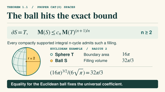
Let be the boundary cycle and its filling. The symbol denotes current boundary, denotes mass, and counts boundary dimensions. Write for the volume of the unit ball in and for the area of the Euclidean unit -sphere. The theorem guarantees an integral current one dimension higher with the following bound.
The exponent comes from scaling. Double every distance and the boundary mass grows by a factor of , while the filling mass grows by a factor of . The coefficient determines how efficiently a cycle can be filled once those units match.
Take the ordinary sphere of radius two in Euclidean three-space. Its area is , and . The bound is exactly the volume of the enclosed ball.
In this example both masses come from ordinary area and volume. For a current, mass also counts the number of sheets present with their absolute multiplicities after cancellation. Two copies of the oriented sphere give a boundary mass of . Two copies of the ball give a filling mass of . The theorem’s upper bound grows by when the boundary mass doubles, while the copied ball’s mass only doubles.
3. Where Previous Isoperimetric Proofs Stopped Short
Almgren established the sharp filling inequality for Euclidean integral currents in arbitrary codimension. Ambrosio and Kirchheim then provided a framework for integral currents in metric spaces, giving a precise meaning to orientation, mass, and boundary even where there are no smooth ambient coordinates.
The CAT(0) setting already had a sharp loop result. Reshetnyak majorization gives a Lipschitz disc bounded by a Lipschitz loop with parametrized area at most the squared length divided by . Wenger gave the Euclidean growth exponent for higher-dimensional integral fillings, with dimension-dependent constants. Schulze obtained the sharp model comparison for two-cycles in smooth Cartan–Hadamard manifolds, including higher codimension. The smooth domain problem also had earlier low-dimensional proofs and results under additional hypotheses. The challenge here was to preserve the exact Euclidean coefficient for all the cycles in the theorem, including those in singular ambient spaces. A comparison that loses a fixed factor can recover the scaling exponent and still miss that coefficient. For the smooth domain problem, the manuscript traces the earlier three- and four-dimensional results to Kleiner and Croke. It also cites Chen, Ghomi and Wang’s comparison in dimensions three through nine.
4. Why CAT(0) Geometry Can Handle Singular Boundaries
A geodesic triangle in a CAT(0) space has a Euclidean comparison triangle with the same side lengths. Between points at corresponding positions on the edges, distances in the space are at most the Euclidean distances. This turns an upper curvature bound into a rule about lengths. It also ensures a unique geodesic between each pair of points, so a deformation toward a chosen center is well defined.
Integral currents combine an oriented, rectifiable geometry with integer multiplicity and a boundary operator. Rectifiability means that countably many Lipschitz charts describe the current up to sets of zero mass. A cycle is a current with zero boundary. Pieces may meet or overlap, with orientation governing cancellation and multiplicity contributing to mass. These features let the theorem address boundaries that cannot be treated as a single embedded smooth hypersurface.
Properness means closed bounded balls are compact. The compact support of lies inside one such ball, and CAT(0) comparison makes the ball convex. Thus the proof can keep the ambient geometry, the cycle, and its filling inside a compact region.
5. Turning a Hypothetical Counterexample Into an Extremizing Cycle
Take a closed convex ball containing the support in its interior. The nearest-point projection to is nonexpansive and fixes the cycle. For any integral -cycle in , let be its minimum filling mass there. Geodesic coning gives a linear upper bound on in terms of boundary mass, and compactness of integral currents gives attainment. If the sharp inequality fails, choose a coefficient low enough that the following functional is positive on a violating cycle.
The linear cone bound controls the masses of a positive maximizing sequence. Weak compactness gives a limit cycle . Filling continuity preserves the filling term, and lower semicontinuity of mass keeps the penalty from increasing in the limit. The positive maximum therefore occurs at a nonzero cycle.
Maximality now restricts how much any competitor can reduce the mass of relative to the cost of filling the difference. The authors rescale distances, which multiplies both terms of the functional by the same factor. They arrange and write for its mass measure.
6. Euclidean Current Charts and the Radial Variation Argument
At almost every point of a rectifiable chart, metric differentiation describes nearby distances by a norm on the chart coordinates. The CAT(0) midpoint inequality passes to that norm and gives the parallelogram identity. The norm therefore comes from an inner product, with a Euclidean volume element in suitable coordinates. This fact supplies the exact mass normalization and later the Euclidean tangent density needed for sharp constants.
Fix a center and write . A nonnegative Lipschitz function specifies how far each point moves toward at small time , leaving the fraction of its original radial distance. This produces both a deformed cycle at fixed time and a current swept by the entire motion. In orthonormal chart coordinates, the spatial portion left after removing the radial differential has determinant . The square root measures the transverse contribution in the swept-mass upper estimate. Here differentiates along the current charts and the dot denotes their inner product on covectors. The determinant is exact for the quadratic comparison form, which bounds the deformed metric. Think of a flat patch in Euclidean space. When the radius points along the patch, the instantaneous motion adds no new transverse direction. When the radius is perpendicular to the patch at the point under consideration, the full radial speed contributes. The square root in the estimate interpolates between those cases without requiring a normal vector field in the ambient space.
Comparing the cycle’s mass decrease with the cost of the sweep gives the radial first variation.
7. The Two-Dimensional Base Case and the Mass Threshold 4π
For cycle dimension two, choose a center of Euclidean lower density. Around almost every point of the cycle, the mass in a shrinking radius- ball has lower limit at least after division by . The unit lower bound on nonzero integer multiplicity is what makes this density estimate independent of the cycle’s sheet count.
Test the radial inequality with . Inside the cutoff ball the derivative of this function vanishes. Outside, putting reduces the difference of the right and left integrands to , bounded above by . The inner contribution is at least and the outer contribution is at most . Taking radii tending to zero for which the separating sphere carries zero mass gives . This forces , contradicting the normalization. The sharp filling theorem for two-cycles is the starting point for the higher-dimensional argument.
8. Higher-Dimensional Induction From Small Fillings to a Sharp Sobolev Inequality
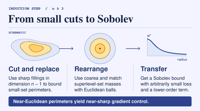
For , cut the extremizing cycle along a superlevel set of a Lipschitz function. Almost every cut has a boundary that is an integral -cycle. Apply the sharp lower-dimensional bound to fill that boundary, and use the filling as a replacement for the removed restriction. If the replacement were much lighter than the piece it replaces, the resulting competitor would violate maximality. Quantitatively, if the removed mass is , the replacement has mass at least for a fixed constant . Together with the sharp filling estimate, this pushes the cut perimeter toward the Euclidean lower bound for small .
Intrinsic coarea expresses the chart-gradient measure in terms of these level boundaries. Rearrangement replaces the levels by concentric Euclidean balls with the same superlevel masses, controlling the gradient energy by the near-Euclidean perimeter estimate. The authors use a mass-transport proof of the radial Euclidean inequality with the sharp Aubin–Talenti coefficient. Rearranging preserves the distribution of values, so the relevant function norms survive the transfer to Euclidean space. Applying the resulting inequality to truncations gives an estimate on the cycle, with an arbitrarily small loss in the leading coefficient and a lower-order term. With , , and norms taken with respect to , it reads
9. Constructing the Critical Sobolev Minimizer
The chart gradient extends by closure in the norm combining size and gradient energy. Compactness in comes from projecting whole weighted currents, then isolating each chart in total variation. Working with the whole current first lets the proof use its zero boundary before restricting to pieces. Strong convergence at the critical exponent requires a further argument because a minimizing sequence could still concentrate.
Minimize the quotient with numerator and denominator . A constant test function gives an upper bound for the infimum, strictly below the Euclidean threshold . Brézis–Lieb splitting separates any residual mass from the weak limit. The almost sharp Sobolev estimate would charge that missing mass at the Euclidean coefficient, so the gap excludes concentration. In the limit, a residual piece carries negligible norm, which eliminates the lower-order term from its estimate.
The nonnegative minimizer can be rescaled so its weak Euler equation has right-hand side when written against test functions. Its weighted mass then satisfies . Moment estimates and power truncations justify the nonlinear tests even where vanishes.
10. Weighted Chords and CAT(0) Variance Give the Final Contradiction
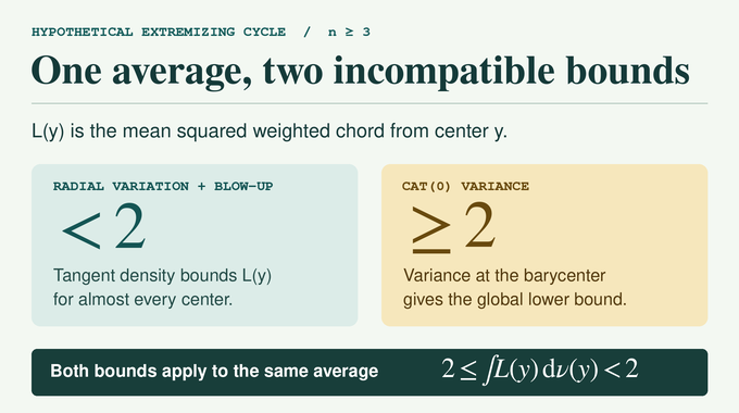
Give the cycle the probability measure . For a fixed center , define the weighted chord and its mean square . Radial variation and the minimizer equation bound the transform by for and centers with . The proof differentiates admissible composite tests, which need no separate gradient for at zeros of .
At large , a blow-up around a typical center gives a Euclidean lower bound for . Integer multiplicity and the stereographic integral fix its coefficient at no less than . Comparing with the transform upper bound yields almost everywhere under .
For the reverse estimate, the proof uses the finite measure with density relative to . Radial variation and the Euler equation give a pointwise lower bound on the squared-distance moment for this measure. At its barycenter, CAT(0) variance adds a squared distance from that center. After integration, the added term equals the barycenter’s own moment, doubling the lower bound. For a consistency check, on a unit Euclidean sphere with , the weighted chord is the usual chord, its mean square is two, and . The two uses of the weight fit together because the chord is squared. Each endpoint contributes an extra factor of the minimizer to the power , which converts the probability density at that endpoint to the density used in the barycenter argument. Both estimates now apply to the same average for the supposed counterexample.
11. What the Proof Establishes for Cartan–Hadamard Domains
Let be a bounded smooth domain in a Cartan–Hadamard manifold of ambient dimension . Its oriented volume current has boundary mass equal to the area of . Apply the filling theorem with . The difference between the supplied filling and the volume current would be a compactly supported, top-dimensional cycle. Such a cycle vanishes because its multiplicity is constant on the connected ambient manifold and zero outside the support. Thus the filling mass is the actual volume of . Rearranging gives the Cartan–Hadamard isoperimetric inequality.
For relatively compact sets of finite perimeter in these dimensions, the boundary current has mass equal to the perimeter, so the same argument applies. The classical surface inequality completes the smooth-domain statement in ambient dimension two. The same uniqueness argument makes the Euclidean ball the only compactly supported integral filling of its oriented sphere in Euclidean space of the ball’s dimension, establishing optimality of the coefficient. A general equality classification and extensions with a prescribed filling topology are separate questions. The theorem’s scope is compactly supported integral cycles in proper CAT(0) spaces.
The Cartan–Hadamard conjecture thus follows from a statement that also governs singular geometry. Euclidean tangent density sets the sharp local scale, and CAT(0) variance constrains how the extremizing cycle fits together globally. Follow Binary Verse AI for more research explainers on curvature, sharp geometric inequalities, and machine-checked mathematics.
What does the Cartan–Hadamard conjecture actually say?
It asks whether domains in complete, simply connected Riemannian manifolds of nonpositive sectional curvature satisfy the sharp Euclidean isoperimetric inequality. OpenAI proves the domain bound in dimensions three and higher through a more general theorem on integral-current fillings in proper CAT(0) spaces. The surface case was already classical.
What is a CAT(0) space, and why does nonpositive curvature matter?
A CAT(0) space is a geodesic metric space whose triangles are no thicker than their Euclidean comparison triangles. This gives the proof distance and convexity estimates even in singular spaces.
What is an integral cycle, and what does it mean to fill one?
An integral cycle is an integer-multiplicity geometric current with zero boundary. Filling it means constructing a current one dimension higher whose boundary is that cycle. Mass measures geometric size, accounting for multiplicity.
Why is OpenAI’s Euclidean filling coefficient called sharp?
The oriented boundary of a Euclidean ball attains the bound. Its ball is the unique compactly supported integral filling in the Euclidean space of the ball’s dimension. This proves the universal coefficient is optimal. A general classification of equality cases is a separate question.
How does OpenAI’s proof improve upon earlier filling inequalities?
Earlier higher-dimensional filling estimates in general CAT(0) spaces gave the Euclidean mass-growth exponent with dimension-dependent constants. OpenAI combines extremizing cycles, radial variation, sharp Euclidean Sobolev estimates, and CAT(0) variance to establish the optimal universal coefficient.
Does the theorem apply in every dimension and to nonsmooth spaces?
It applies to compactly supported integral cycles of every dimension from two upward in proper CAT(0) spaces, including singular spaces. Ambient dimension and integer multiplicity are unrestricted. The theorem concerns integral-current fillings, whose topology is unspecified.
What part of the Cartan–Hadamard proof is verified in Lean?
The Lean scope documentation identifies two formalized results: the sharp integral filling inequality and optimality of its Euclidean coefficient. The manuscript also contains the domain corollary and an expository proof of the filling theorem.