
A sphere can be changed by an arbitrarily small smooth deformation and yet support Laplace eigenfunctions with far more nodal area than Yau nodal conjecture permits. In a September 2026 manuscript, OpenAI constructs one fixed metric on the three-sphere and another on whose exact eigenfunctions have nodal measures growing faster than any constant multiple of . The result disproves the smooth upper-bound prediction in dimensions three and four, not its lower bound or the analytic-metric theorem. The decisive advance is a method for manufacturing many stable zero crossings and preserving them while correcting approximate waves into exact eigenfunctions.
Table of Contents
1. What Is Yau’s Nodal Conjecture, and What Does Its Upper Bound Predict?
For a closed -dimensional Riemannian manifold with metric , a real nonzero Laplace eigenfunction obeys the equation below. Its nodal set is the collection of points where the function vanishes. The quantity measures its intrinsic -dimensional Hausdorff size: length on a surface and area in three dimensions.
Yau predicted that, for each fixed smooth metric, this size stays between two metric-dependent multiples of the frequency scale . The conjecture comprises two separate inequalities:
| Question | Result in the paper |
|---|---|
| Object measured | Intrinsic Hausdorff measure of eigenfunction zero sets |
| Setting | Fixed smooth metrics on S³ and S² × T² |
| Three-dimensional conclusion | Nodal area / √eigenvalue becomes unbounded |
| Four-dimensional conclusion | Nodal 3-volume / √eigenvalue becomes unbounded |
| What survives | Lower estimate and real-analytic sharp bounds |
2. Why the Nodal Upper Bound Resisted Proof for Smooth Metrics
Donnelly and Fefferman proved the sharp square-root estimates for real-analytic metrics in 1988. Smooth metrics provide fewer quantitative controls on oscillation. Hardt and Simon established a general non-polynomial upper bound, while Logunov later obtained a polynomial bound in dimensions at least three and proved the sharp smooth lower estimate. Those results did not supply the conjectured upper exponent.
This is a problem in spectral geometry, not merely the topology of zero sets. An eigenfunction may have intricately connected nodal components without their total measure exceeding the proposed rate. Related questions about where an eigenfunction reaches its extrema appear in work on the hot spots conjecture, but the present paper concerns the quantitative size of zeros. The upper-bound gap existed because available estimates could not preclude excessive nodal measure for arbitrary smooth coefficients.
3. OpenAI’s Proof: The Counterexamples in Dimensions Three and Four
Theorem 1.1 says that every neighborhood of the round metric on contains a smooth metric and a sequence of exact real eigenfunctions with positive eigenvalues tending to infinity, for which the normalized nodal area diverges. Theorem 1.2 gives an analogous fixed metric on , with three-dimensional nodal measure.
The constant in Yau’s proposed bound may depend on the metric. Therefore constructing a different metric at every frequency would be insufficient. Both the fixed-metric requirement and exact eigenfunction equation are essential. Near-round means arbitrarily close in the smooth topology, not that the unperturbed round sphere violates the theorem. The 60-page original manuscript states these claims as Theorems 1.1 and 1.2.
4. The Three-Sphere Construction: Starting From Exact High-Frequency Waves
On the standard three-sphere in Euclidean four-space, let . The harmonic polynomial behind the construction restricts to an exact round-sphere eigenfunction. Its azimuthal oscillations are transparent, and its radial size is approximately , which makes it a useful background signal outside the modified region.
Inside a chosen coordinate cube, the authors introduce an envelope , with a reference profile . The inequalities in an inner region and outside it separate the added packets from the background wave. Perturbations remain compactly supported, preserving a clean outer annulus for later correction. Importantly, each envelope is selected before the frequency is increased.
5. Corrugated Envelopes: How the Proof Amplifies Nodal Complexity
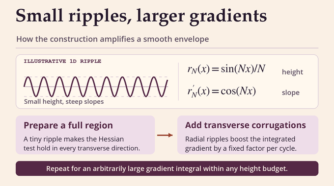
The geometric engine is Proposition 2.2. Write , and . A strict profile admits a transverse vector with , and a positive Hessian trace in the two chosen directions:
That positivity is the condition needed to fit complex phases underneath the envelope. It looks restrictive: violent corrugations increase derivatives and could destroy it. The authors avoid this by a two-stage cycle. Tiny high-frequency one-variable ripples first produce a region where the Hessian inequality is positive for every allowable transverse direction, called a full region. Periodic averaging guarantees that this region captures a definite fraction of the gradient mass.
They then use a radial periodic perturbation in two variables transverse to , of schematic form . The amplitude tends to zero as increases, while its transverse gradient contribution stays of order . On a fixed fraction of annular cells, the new gradient is uniformly larger. A favorable tangential Hessian term of order protects strictness, including transition regions where cutoffs vary.
Each full cycle multiplies the integral by at least a fixed factor greater than one. Repeating finitely many cycles makes that integral arbitrarily large while the total change in the profile remains arbitrarily small in . The profiles are smooth, but their higher derivatives need not be uniformly controlled across cycles. Crucially, the later wave estimates allow their frequency threshold to depend on the chosen profile.
6. Complex WKB Waves: Building Approximate Eigenfunctions With Controlled Errors
For a selected strict envelope, Section 3 builds localized complex geometrical-optics packets. A packet has the form , with complex phase , cutoff , and a finite inverse-frequency transport expansion . The leading phase satisfies a complex eikonal equation, while successive Taylor coefficients cancel the remaining phase and transport errors to prescribed finite order.
The second estimate is local, with now denoting distance from a packet center. It forces Gaussian localization on the frequency-dependent transverse scale. An admissible complex Hessian is selected below , and the strict trace inequality guarantees that choice. A finite Taylor recursion then produces any requested residual accuracy in the weighted norm, rather than pretending to solve the exact eikonal equation globally.
These are quasimodes, not yet Laplace eigenfunctions. Specifically, the residual and its finitely many derivatives can be bounded by for any preassigned . The construction chooses the finite jet orders first and increases afterward. That order of choices is what eventually makes arbitrarily small metric corrections possible.
7. From Sign Changes to Nodal Area: The Geometric Counting Argument
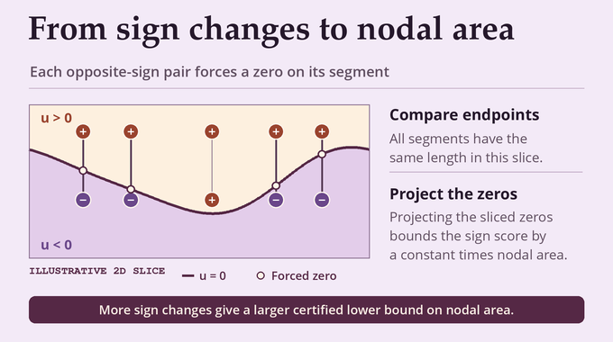
A sum of Gaussian-weighted packets is added to . The authors do not simply equate expected nodal area with a random-wave heuristic. Instead they choose one realization with an explicitly measurable collection of opposite-sign comparisons. Divide the coordinate cube into small subcubes; in each coordinate direction compare values at points separated by , where approximates .
Every strict opposite-sign comparison forces at least one zero in the intervening segment. Slicing into coordinate slabs and projecting their zeros bounds the score by a metric-uniform multiple of nodal area, even if the zero set is singular. At the same time, the covariance calculation for nearby Gaussian values shows that some wave realization has a score at least a constant times . This translates the corrugated envelope’s large integrated gradient into large nodal area.
A second probabilistic estimate prevents simultaneous cancellation of the real value and gradient, using several phase directions and one displaced packet. In scale-adjusted form their pair has a polynomial lower bound everywhere. Strict opposite signs are lower semicontinuous under uniform convergence, and multiplying by a positive function does not change them. Those two properties make the score a durable witness during exactification and later metric limits.
8. How the Three-Dimensional Proof Turns Quasimodes Into Exact Eigenfunctions
An approximate eigenfunction fails to solve the exact equation by a small residual . Lemma 4.1 absorbs this defect into a positive scalar conductivity and an independent density , obtaining . The value–gradient noncancellation estimate makes the denominators in the corrections safe. Unlike familiar coefficient-recovery questions in the Calderón inverse problem, here conductivity is deliberately adjusted to realize a chosen oscillatory function.
But arbitrary and do not describe an ordinary metric. In dimension three, the scalar conductivity metric construction requires a determinant compatibility relation. The authors divide by a positive function and obtain new coefficients and . Enforcing leads to a semilinear elliptic equation:
A contraction argument near solves it, exploiting the positive linearized operator . The factor is cut off to recover the original wave in an exterior annulus. That cutoff creates a residual determinant defect, but not an equation defect. The solution is a tensor repair on the two-plane orthogonal to , scaling only those transverse directions until while keeping . The resulting metric has exactly the desired Laplacian and the positive division preserves all zero sets and signs.
9. The Four-Dimensional Construction on S² × T²
The second branch is not a product trick applied to the first. On the product of a round two-sphere and a flat two-torus, the authors start from separated exact modes. For spherical latitude , angular coordinate and circle coordinate , the background eigenfunction and eigenvalue are:
Here the unperturbed logarithmic envelope is . Its strictness condition uses rather than the three-dimensional expression. A favorable transverse Hessian direction exists inside the three-dimensional orthogonal complement of . Alternating preparation with transverse radial corrugations again makes arbitrarily large, while positive and negative envelope gaps isolate the active patch from the fixed background.
Section 8 constructs localized packets on a frequency-dependent lattice, with three independent imaginary phase directions. A displaced packet supplies an additional real direction, preventing simultaneous cancellation of value and all four first derivatives. The authors then obtain a stable sign score comparable from below to . The analogy with the first branch is deliberate, but the higher-dimensional transversality and next metric correction are different.
10. Why Dimension Four Needs a Different Exactification Argument
In four dimensions, Lemma 10.2 first repairs the quasimode using a small symmetric contravariant tensor and independent density increment . Their formula divides by where it is safely nonzero and by where the gradient is safely nonzero, with smooth cutoff functions making the two cases compatible. This yields an exact weighted eigenfunction equation, not yet an ordinary Laplace–Beltrami eigenpair.
After redefining the metric, the density weight is conjugated away with a positive square-root multiplier. The resulting equation contains a small potential . Dimension four permits a particularly useful conformal change with , provided the scalar factor solves:
Linearizing around gives , which has a uniformly controlled inverse in the required Sobolev norms. This coercive negative operator avoids any spectral nonresonance assumption. The argument resembles other careful uses of nonlinear elliptic estimates, such as those studied in the De Giorgi problem, without importing a result from that separate work.
Cutting off restores an untouched exterior but breaks a volume-determinant relation on a collar. There the nonvanishing background derivative defines a rank-three projection onto the tangent directions of level sets. The authors adjust only this tangent bundle until the contravariant tensor has determinant and still sends to the same flux. The equality of volume and divergence then makes an exact eigenfunction. A positive multiplier preserves its signs, as in dimension three.
| Proof component | Three-sphere | S² × T² |
|---|---|---|
| Weighted correction | Scalar conductivity and density | Tensor conductivity and density |
| Positive factor | Semilinear factor v and division U/v | Conformal factor Z and division v/Z |
| Compatibility | Metric determinant det A = d | Contravariant determinant = ρ² |
| Final repair | Two tangent directions on a clean annulus | Three tangent directions on a clean collar |
11. One Fixed Smooth Metric: Simplicity, Stability, and the Final Limiting Proof
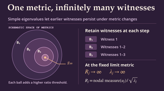
At each frequency, exactification so far gives a nearby metric with one impressive eigenfunction. To defeat Yau’s metric-dependent constant, the paper must retain infinitely many such witnesses for the same eventual metric. A multiple eigenvalue makes an individual eigenfunction unstable under perturbation. Sections 5 and 11 therefore create a localized, volume-preserving tensor perturbation tangent to the selected eigenfunction’s level sets. It leaves that function an exact eigenfunction while splitting its eigenvalue from the remaining eigenspace.
Near a simple eigenvalue, normalized eigenfunctions vary smoothly with the metric. Because the sign score is lower semicontinuous and uses strict comparisons, each nodal-area witness survives throughout some open neighborhood of metrics. The construction chooses a new very high frequency and metric inside the previous neighborhood, obtains a larger score, and shrinks to a closed ball contained in all previous persistence sets.
Nested balls of decreasing diameter converge in the complete space of metric tensors to a smooth positive metric . Every earlier witness continues to exist there, with its own slightly shifted exact eigenvalue. In the three-sphere proof the increasing frequency windows are disjoint, so the eigenvalues diverge. In the four-dimensional proof the limiting argument similarly imposes growing eigenvalue and score thresholds. This is why an unbounded normalized ratio is proved for one metric rather than merely for a sequence of changing metrics.
12. What the Counterexamples Settle and What They Leave Intact
The Yau nodal conjecture has two sides. This paper refutes the smooth upper bound in dimensions three and four, while the sharp lower bound survives. Donnelly–Fefferman’s analytic-metric estimates remain compatible: a metric can be arbitrarily close to analytic in the smooth topology without itself being analytic. The separate surface result cited by the authors establishes the smooth upper estimate in dimension two, and the three-dimensional construction extends qualitatively to higher dimensions by taking products.
The conclusions do not assert for a fixed positive in dimensions three or four. The stronger power-law result belongs to a companion paper. OpenAI’s Family 350 formalization scope describes theorem-level counterexamples on both manifolds, while the Lean source exposes the formal statements. The 60-page manuscript supplies the detailed analytic construction. These should not be conflated into a claim that every intermediate WKB calculation was independently formalized.
For spectral geometry, the lesson is exact: high-frequency nodal measure can be amplified by a smooth metric perturbation while exactness and one fixed background metric are maintained. Binary Verse AI will continue examining the equations and proof architecture behind results like this. Explore our infinity-Laplacian regularity analysis for a different example of how smooth PDE geometry hinges on a precise technical condition.
1. Has Yau’s nodal conjecture been disproved?
Its upper-bound prediction fails for certain fixed smooth metrics in dimensions three and four. The lower bound remains intact, and the real-analytic case is not contradicted.
2. What is Yau’s nodal upper-bound formula?
For eigenfunctions with eigenvalue λ, the prediction was ℋ_g⁽ᵈ⁻¹⁾(Z_u) ≤ C_g√λ. The constant depends on the fixed metric, not on the eigenfunction or eigenvalue.
3. How can a metric close to the round sphere violate the upper bound?
The proof constructs smooth metrics arbitrarily close to the round metric in the C∞ topology while producing eigenfunction sequences with unbounded normalized nodal area. It does not claim that the round metric itself violates the bound.
4. Why does the counterexample require one fixed metric?
Yau’s conjecture permits a different constant for each metric. Changing the metric at each frequency would not disprove the existence of such a constant for any single metric.
5. Are the counterexample eigenfunctions exact or approximate?
They are exact eigenfunctions in the final theorem. The proof first constructs highly accurate quasimodes, then corrects both the eigenfunction and metric while preserving the relevant sign changes.
6. Does OpenAI’s proof establish power-law growth beyond √λ?
No. This paper proves an unbounded ratio to √λ, not an excess of the form λ^(1/2+ε) for a fixed positive exponent. That stronger result belongs to a separate companion paper.
7. What does the Lean formalization verify about the counterexamples?
OpenAI’s Family 350 scope document lists formalized counterexample statements for the three-sphere and S² × T². The detailed mathematical arguments are presented in the manuscript; the article distinguishes them from the selected formal statements.