
In a complete graph on four vertices, a star is a perfectly good spanning tree. Yet it uses all three edges that leave its center. The thin tree conjecture asks how sparse a single spanning tree can be across every cut when the original graph is highly connected. In a September 23, 2026 preprint, OpenAI proves that a deterministic polynomial-time algorithm can find a tree that uses at most of the edges across each cut of any finite -edge-connected loopless multigraph, for a universal constant . The guarantee applies to the same output tree across all cuts, even when the input stores parallel-edge counts in binary.
Table of Contents
1. What Is the Thin Tree Conjecture? Understanding the All-Cut Condition
| Item | Guarantee |
|---|---|
| Input | Finite, undirected, loopless multigraph with edge connectivity at least . |
| Output | One spanning tree using at most a fraction of the original edges across each nontrivial cut. |
| Running time | Deterministic and polynomial in the binary input length, with explicit edges or binary multiplicities. |
| Sharpness | Two vertices joined by parallel edges force the fraction . |
A spanning tree connects all vertices without cycles and uses edges. For a nonempty proper vertex set , the cut contains every edge with one endpoint in and the other outside it. Each parallel copy counts separately. A graph is -edge-connected if every such cut contains at least edges. A spanning tree is -thin if for every nontrivial .
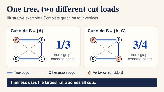
In the four-vertex example, isolate vertex A. The star retains all three edges across that cut, while the path retains just one. Change the cut to the alternating vertices A and C, and all three path edges cross, out of four graph edges. The same path therefore has ratios of and on these two cuts. The objective measures the worst ratio over every choice of vertex set.
2. The Strong Thin Tree Conjecture and the Inverse-Connectivity Bound
Goddyn’s qualitative conjecture asks whether, for each positive thinness target, sufficiently large edge connectivity guarantees a tree meeting that target, with a threshold independent of the vertex count. The strong thin tree conjecture specifies the rate. A single absolute constant should suffice for all graphs, with the guaranteed fraction shrinking in inverse proportion to .
Take two vertices joined by parallel edges. There is one cut up to exchanging its sides. All copies cross it, and every spanning tree selects exactly one copy. Its cut ratio is exactly . As grows, this family rules out a universal bound of smaller asymptotic order. It also shows why parallel edges belong in the theorem: the connectivity can grow while the vertex count stays fixed. The lower bound establishes the rate, leaving the best universal constant as a separate question.
3. Earlier Thin-Tree Bounds and Their Scope
The maximum-entropy spanning-tree rounding of Asadpour and colleagues gave the constructive thinness scale . The extra factor depends on the number of vertices. Anari and Oveis Gharan improved the existence bound to for general multigraphs and developed the effective-resistance and hierarchy methods that the new work extends. Their bound still depends on and comes from an existence proof.
For planar graphs and graphs on a fixed orientable surface, Oveis Gharan and Saberi had already obtained constructive inverse-connectivity bounds. Other results focus on the cuts themselves. Klein and Olver handle a prescribed laminar family, where any two sets are nested or disjoint. Klein, Olver, and Yeoh construct a tree that crosses each cut smaller than at most 88 times. The new result removes the dependence on graph order in the general all-cut setting and gives a deterministic construction.
4. OpenAI’s Polynomial-Time Theorem
Theorem 1.1 takes a finite, undirected, loopless multigraph on at least one vertex and a positive integer for which is -edge-connected. There is a universal constant such that the deterministic algorithm returns a spanning tree satisfying
The input may list labeled edge copies explicitly or give endpoint pairs with binary-encoded nonnegative integer multiplicities. The running time is polynomial in the total binary input length in either representation. On one vertex the algorithm returns the empty tree, and the cut condition is vacuous. The companion preprint proves existence and supplies the hierarchy geometry. The algorithmic paper turns that approach into a finite search with rational arithmetic and controlled precision. Both preprints appear in OpenAI’s October mathematics release.
5. Why Spanning Tree Packing Alone Falls Short
The Nash–Williams–Tutte theorem characterizes when a graph has edge-disjoint spanning trees. For each partition of the vertices, the number of edges joining distinct parts must be at least . Each tree needs at least such edges to join the parts, and the theorem makes the condition sufficient. Summing the connectivity bounds on all parts counts each crossing edge twice. This gives at least disjoint trees for a -edge-connected graph, with one tree available by connectedness when .
For a fixed cut, disjointness caps the average tree load at the graph’s cut size divided by the number of trees. The tree below that average can depend on the cut. The construction instead selects a subgraph that reduces every cut load while retaining a large packing.
6. Metric-Cone Shortcuts and Effective Resistance
Work in the subspace perpendicular to the all-ones vector. For an oriented edge , let be the difference between the coordinate unit vectors at its endpoints. The graph Laplacian sums the outer products of these incidence vectors. A shortcut matrix is positive definite on that subspace and assigns each edge a resistance . With the Laplacian in place of , this is the usual effective resistance for unit edge conductances.
The algorithm uses a metric test cone of centered positive semidefinite matrices whose squared distances obey the triangle inequality. A centered cut indicator gives a rank-one member of this cone. In the feasible set for , the trace pairing against every such test is bounded above by three times the pairing with . In particular, evaluating on a centered cut indicator gives at most three times the cut size.
The hierarchy proof uses a second geometry for the same vertex labels. It doubles the metric space, placing each point opposite a partner so their distances from any profile point sum to a common constant. In the convex hull of distance profiles, radii are affine. Moving toward a center or its partner changes the radius by exactly the distance traveled. This lets the proof trim balls into shells and charge their widths to lengths of graph edges crossing them. The charging bounds control average resistance on marked hierarchy boundaries, providing a simultaneous geometric response to nested partitions.
7. Convex Capacity Ramps and Low-Resistance Tree Packing
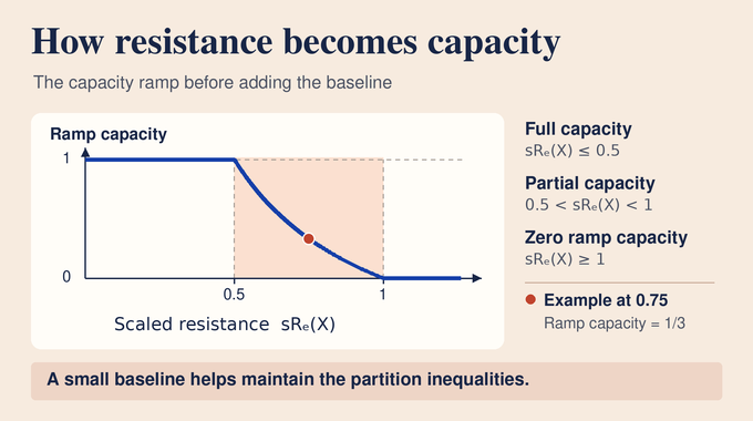
A hard resistance threshold can discard many edges at once and destroy a packing. Section 3 assigns continuous capacities instead. At a positive parameter , an edge gets full ramp capacity when , zero when , and a continuously varying capacity in between. A small positive baseline keeps capacities available for the partition argument. The algorithm raises gradually while updating and lowering the target packing size by a controlled amount.
Partition inequalities require sufficient total capacity between the parts of every partition. Uncrossing reduces a hypothetical obstruction to a chain of nested partitions, where the geometric response works simultaneously. Exact rational separation checks the constraints without listing every partition. The oracle trades the partition test for inequalities involving minimum spanning tree lengths.
A minimum spanning tree computation can then expose a violated tree constraint in the rational linear program used by the oracle. The proof supplies a quantitative interior ball for the ellipsoid method and a rounding margin that keeps the output rational and feasible. At the last step, dropping the baselines loses less than one unit across any partition. Graphic-matroid union then extracts actual edge-disjoint trees from the active edges. In a graphic matroid the independent edge sets are forests, and the spanning trees of a connected graph are its matroid bases.
Proposition 3.1 starts with disjoint trees in an explicitly listed multigraph on at least two vertices, for at or above an absolute threshold. It returns a rational shortcut and a packing of trees with
Here is absolute, and the resistance bound applies to every edge in the returned packing.
8. Rank-Preserving Normalization Through Sparsification
The cut representation alone gives no lower bound on how many edges survive between the parts of an arbitrary partition. Section 4 builds a second vector system from the union of the trees. It drops one row of the incidence matrix, chooses positive edge weights by approximate minimization of a log-determinant objective, then whitens the weighted columns. Whitening is a common linear change of coordinates that makes the sum of their outer products the identity.
The derivatives of the objective are weighted edge leverage scores minus . A small gradient makes each squared vector norm at most . Positive column scalings and a common invertible map preserve the rank of every subset of incidence columns. For a partition into parts, the internal edges then span at most dimensions. At least dimensions are available to test the crossing edges. This is how the frame turns a lower bound on retained covariance into a lower bound on the number of retained edges across each partition.
9. Certified Matrix Signing Selects the Edges
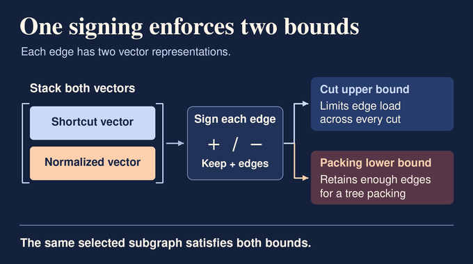
For each edge in the packing, the algorithm stacks the shortcut vector above the rank-preserving vector . The shortcut bounds the squared norm of the first block, and normalization bounds the second. One signing therefore acts on both representations of the same edge. The positive signs identify the edges to keep. A signing bounds the deviation of the selected outer-product sum from half the original sum. Because the two representations share one sign per edge, the algorithm produces a single subgraph that satisfies both matrix estimates.
The stack can contain irrational entries, so Section 5 approximates scaled copies of the columns by rational vectors. It decomposes the positive semidefinite residual into rational outer products and adds padding to complete the covariance exactly to the identity. Extra coordinates let the proof control the effect of discarding the padding after signing. Appendix A gives a finite-bit implementation of the rank-one signing method of Ezeunala and Jiang. An exact rational positive semidefinite test certifies the selected set, with a proved allowance for approximation error. The resulting covariance is within of half the original stacked covariance in operator norm, for an absolute constant .
10. Repeated Sparsification Produces One Thin Tree
Lemma 6.1 uses the two diagonal blocks of the certificate differently. The upper bound on the shortcut block limits the load on each cut to a fraction of its previous size. The lower bound on the normalized frame, projected onto the directions left by the internal edges of each partition, certifies a surviving packing of size . It lies between and and is close enough to half that
Here is absolute. Multiplying the bounds over the rounds telescopes the packing ratios to the final packing size divided by the initial one. The extra factors also have a bounded product. Read the packing sizes backwards: each earlier size is at least twice the next. The sum of their inverse sixteenth powers is bounded by a geometric series, and the logarithm of the product is bounded by a constant times that sum.
The initial packing has size at least . The algorithm stops once the packing size is below a fixed absolute threshold and still at least one. Any spanning tree of the final connected graph inherits its cut upper bounds. This yields the inverse-connectivity guarantee without a graph-size factor from the number of rounds.
11. Binary Multiplicities, Cost-and-Cut Rounding, and the Result’s Limits
Expanding a binary multiplicity can take exponential space. Section 6 first caps each endpoint pair’s count at . A cut still has capacity at least : either one capped pair contributes , or every crossing count stays the same. The algorithm multiplies the capped counts by and rounds down. A cut crosses at most unordered pairs, so the rounding loss leaves at least edges on every cut. The auxiliary graph has fewer than explicit edges. Its cut sizes are bounded above by the original sizes times . A tree uses at most one copy per pair, so each selected pair lifts to an original edge. The auxiliary bound of becomes in the original graph, with the factor two absorbed into the universal constant.
Corollary 7.1 takes a finite undirected graph on at least two vertices with explicitly listed edge records, allowing loops and parallel records. Nonnegative rational masses and costs are given in binary, with total mass on every nontrivial cut. Fix an integer . In polynomial bit time it finds a spanning tree in the positive support, with total tree cost , satisfying both
The cut bound holds for every nontrivial . The proof compresses fractional masses into integer multiplicities and, for large enough instances, repeatedly extracts and deletes thin trees. Selecting the cheapest uses disjointness to bound cost by the average, with the cut estimates already guaranteed. Costs need no metric assumption. When several parallel records share endpoints, the proof combines their fractional masses and uses the cheapest positive-mass record when lifting the selected tree. This preserves the fractional mass on every cut before rounding and can only lower the fractional cost charged to that endpoint pair. This thin-and-cheap rounding is relevant to asymmetric traveling salesman relaxations. Constant-factor ATSP algorithms already existed, and the paper gives no new approximation ratio for that problem or implementation benchmarks for thin-tree construction.
The thin tree conjecture thus has an algorithmic resolution whose defining feature is the coupling of cut control with packing preservation. Follow Binary Verse AI for more research explainers on graph algorithms, including maximum-cardinality matching, graph coloring, and graph isomorphism tests. For this result, OpenAI’s Lean scope covers the existence bound and the deterministic polynomial-time guarantee for explicit and binary-multiplicity inputs. The Lean proof module is separate from the comparator statement. The scope document describes these guarantees at the theorem level.
12. Frequently Asked Questions
Has the thin tree conjecture been proved?
Yes. OpenAI’s September 2026 preprints prove the strong form and give a deterministic polynomial-time construction. For a finite k-edge-connected loopless multigraph, the algorithm finds one spanning tree that uses at most a C/k fraction of the edges across every cut, for a universal constant C. The construction appears in a preprint.
What is the difference between a thin spanning tree and a minimum spanning tree?
A minimum spanning tree minimizes total edge weight. A thin spanning tree limits the fraction of graph edges it uses across each cut. A minimum-cost tree can still use a large share of the edges across a particular cut.
Why does the algorithm need more than a packing of edge-disjoint spanning trees?
A large packing bounds the average tree load on each fixed cut. The tree below that average can differ from cut to cut. The new construction repeatedly selects subgraphs that control every cut and retain enough edge-disjoint trees. Any spanning tree of the last connected subgraph then inherits its cut bounds.
How does the algorithm control exponentially many graph cuts?
It uses partition inequalities, convex optimization and matrix certificates. Minimum spanning trees provide a separation routine for the partition constraints. A matrix bound then applies to every cut by evaluating it on centered cut indicators, while graphic-matroid union recovers the edge-disjoint trees.
Is the strong thin tree algorithm polynomial-time even with enormous edge multiplicities?
Yes. The running time is polynomial in the number of bits used to encode the input. For a graph on n vertices, the algorithm truncates, rescales and rounds the binary multiplicities to make an auxiliary graph with fewer than n⁴ explicit edges. It then lifts the chosen tree edges back to the original graph.
Is OpenAI’s strong thin tree proof formally verified in Lean?
Yes, at the level of the released theorems. The published Lean scope covers the existence bound and the deterministic polynomial-time construction, including the binary-multiplicity runtime guarantee. These are theorem-level guarantees. The scope document describes the formal results, and the proof module is separate from the comparator statement.
Does the proof produce a better approximation algorithm for asymmetric TSP?
No. The paper proves simultaneous thin-and-cheap rounding for rational fractional cut inputs, a technique relevant to asymmetric traveling salesman relaxations. Its stated guarantees bound the cost and cut loads of a spanning tree. Constant-factor algorithms for asymmetric TSP were already known.