
How long can a network avoid both five mutually connected vertices and a large group with no connections among them? For the Ramsey number , the power of had been settled, but the best bounds still differed by three powers of a logarithm. OpenAI’s September 24, 2026 preprint pins the logarithmic exponent down to three, giving . The new Ramsey number bounds come from showing that a graph built from projective geometry can have much smaller independent sets than the previous analysis guaranteed. The proof turns any putative long independent sequence into a message shorter than its entropy permits. Read the original preprint.
Table of Contents
1. Ramsey Number Bounds and the Problem r(5,t)
A clique is a set whose vertices are all pairwise adjacent. An independent set is a set with no edges between its vertices. In a network where edges represent mutual acquaintance, these are groups of mutual acquaintances and mutual strangers. The Ramsey number is the least vertex count at which every simple graph contains a five-clique or an independent set of size . The two targets can differ, making these off-diagonal Ramsey numbers.
For a lower bound, exhibit one graph that avoids both patterns. For an upper bound, show that every graph beyond a threshold must contain at least one. Theorem 1.1 improves the lower bound and recovers the classical upper bound.
| Threshold | Five-clique or independent set of size |
|---|---|
| Sharp exponent | Three in the logarithmic denominator of |
| Previous lower bound | up to a constant factor |
| New ingredient | Short descriptions of sparse point–hyperplane pairs |
| Result scope | Asymptotic bounds for all sufficiently large integers |
2. What OpenAI’s Proof Establishes About r(5,t)
For every fixed and all sufficiently large integers , Theorem 1.1 gives the following bounds, where is an absolute positive constant and denotes the natural logarithm.
The threshold for can depend on . Taking logarithms turns each power of into a multiple of . Subtracting from removes the leading power of , giving the limit that defines the sharp exponent.
Equivalently, the denominator is , with denoting a quantity that tends to zero. A vanishing exponent error can still give an unbounded multiplicative factor. For example, an error of gives the factor .
3. Why Earlier Bounds Left a Logarithmic Gap
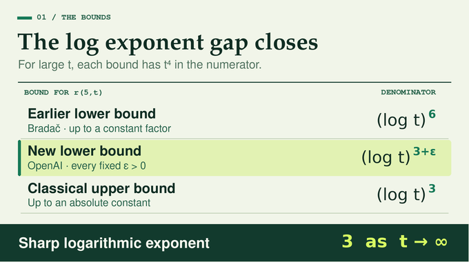
Spencer’s local-lemma argument gave a Ramsey number lower bound on the scale . Bohman and Keevash improved the logarithmic loss using the random clique-free process, reaching up to a constant. Both bounds still had a cubic power of . Finite geometry supplied a different route. Mattheus and Verstraëte used a Hermitian unital for , and Bradač’s projective construction reached the fourth power for .
Bradač’s lower bound was proportional to , while the classical Ramsey number upper bound had in the denominator. Their scales differed by a factor of , ignoring constants. OpenAI’s Ramsey proof uses the ordered flag graph from Bradač’s work and improves the analysis of the independent sequences it can contain. Read Bradač’s off-diagonal Ramsey paper.
4. The Classical Upper Bound and the Three Logarithmic Gains
In a triangle-free graph, a vertex’s neighbors form an independent set. If no independent set reaches size , every degree is below . The paper proves a stronger independence estimate than the greedy bound by choosing a uniformly random independent set. Conditional on the choice outside a vertex’s closed neighborhood, the completions are either the vertex alone or any subset of its available neighbors. Averaging gives a logarithmic improvement over greedy selection and yields an upper bound for proportional to .
For a graph with no clique of size , each neighborhood has no clique of size . An edge’s common neighborhood has no clique of size . This bounds the maximum degree and the number of triangles through any edge. The paper samples vertices independently, then deletes high-degree vertices and breaks remaining triangles. At high maximum degree, the resulting triangle-free induced graph retains enough vertices relative to its degree for the independence estimate to gain another logarithm. At low degree, greedy selection already suffices. The high-degree step adds a factor of order at each passage, giving for and for .
5. How Projective Flags Rule Out Five-Cliques
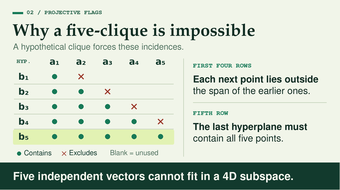
In , a point is a one-dimensional subspace of the five-dimensional vector space over the field with elements. A projective hyperplane comes from a four-dimensional vector subspace. A flag consists of a point and a hyperplane that contains it. The notation means that incidence holds. Each vertex is a position in a stream of independently sampled uniform flags. Repeated flags are allowed because positions are the vertices. For positions , the edge rule is
For a worked example, suppose the first two flags of a proposed clique have point representatives and , the first two standard basis vectors. The first hyperplane contains and excludes . The second hyperplane contains both and must exclude the third point, so that point lies outside their span. Continue in the same way. The fourth hyperplane contains the first four points and excludes the fifth. The five vectors are therefore linearly independent. Yet the fifth hyperplane must contain all five, which is impossible in a four-dimensional subspace.
6. Why a Selected Independent Sequence Has High Entropy
An independent set, read in stream order, gives a consistent tuple. If an earlier point lies on a later hyperplane, the reverse incidence must hold as well. Suppose every stream contains such a tuple of length , and select one by a fixed rule. Here , with fixed and small. The selected tuple can be strongly biased because its selection depends on the entire stream.
The paper bounds the probability of each possible output without treating its coordinates as independent. A particular tuple must occur at some choice of positions. For prescribed positions the probability of a prescribed flag tuple is , with the total number of flags. A union bound over position sets limits the largest atom, and Shannon entropy is at least the negative logarithm of that atom. Write . The flag count scales as , and the stream has positions. For retained lengths comparable to , the logarithm of the number of position choices costs at most . This leaves an excess of , up to an loss, over even after conditioning on events with probability bounded below.
7. Marking Scans, Conditional Dependence, and Collisions
The forward scan keeps, for each potential later hyperplane, the span of the dual vectors representing earlier marked hyperplanes whose points lie on it. Consistency forces the point of a new flag to lie in every hyperplane in that span. A flag is cheap when it belongs to one of the scan’s small, decoder-known classes. In one case, its hyperplane already belongs to many recorded spans. In the other, its point hits relatively few hyperplanes in a tracked rank class. An expensive flag escapes both descriptions, but adding it enlarges enough spans to shrink a tracked set by a fixed fraction of order . Only expensive updates can occur.
A second scan reverses the order and exchanges points with hyperplanes. Recording the scan classes and the expensive flags leaves at most joint options per remaining slot and supplies separate caps on its two endpoints. The proof then partitions windows into representative blocks and middle targets. After revealing older rounds of representatives, it selects a fresh round before reading its values. An entropy chain rule bounds the remaining mutual information between representatives and targets.
Under the actual joint law, an incidence that would create an edge is forbidden. Under the product of the conditional marginals, its probability is bounded by mutual information. Incidences in both directions require an extra geometric argument. Where they can persist, the proof charges pairs lying in rectangles formed by a dual subspace and its annihilator. A uniform bound on stream occupancy makes these collisions rare enough. Nearly uniform levels of the endpoint distributions then supply large, sparse supports for the next step.
8. The Sparse Incidence Description Theorem
In projective dimension , a uniformly random point and hyperplane are incident with probability close to . Theorem 4.1 concerns hidden sets of points and of hyperplanes with density far below that scale, yet with a product of sizes at least for a controlled loss parameter . The decoder knows enclosing sets, while the encoder knows the hidden sets. A short public-table message describes a set that contains a constant fraction of the smaller hidden support and is at most times its size. Here is the theorem’s sampling parameter, with .
A small support can be sent directly by its rank among subsets of the known enclosure. For larger supports, the proof looks for concentrations on planes or hyperplanes. A large cell lets it restrict points and hyperplanes to a proper flat and invoke the description theorem in lower dimension. Hyperplanes can have the same restriction, so the proof groups restrictions by the number of original hyperplanes that lift them.
When the cells are small, the encoder sends the flat lists and counts instead. Polynomial bounds on rich lines and estimates for overlapping hyperplanes control how often several hyperplanes through the same query point share many training points. This controls the dependence that remains when those hyperplanes are tested against the same random batches.
9. How the Poisson Score Detects Sparse Structure
In the small-cell case, the predictor draws independent batches from the training set with Poisson-distributed sizes. This makes sample counts independent across points and batches. Hyperplanes can still share samples, so their emptiness events can be correlated. The score examines hyperplanes through the query point, using empty-batch indicators and a centering term adjusted for its assigned cells. The centering reduces the contribution from typical hyperplanes. A hyperplane is exceptional if its training incidence departs sufficiently from the expected mass, either across the whole training set or within a recorded cell. The exceptional hyperplanes empty in every batch supply the main signal.
Sparse incidence provides many candidates for those empty exceptional hyperplanes. On successful rows, incidence variance separates the typically low training counts from higher ambient counts. The proof controls score errors with a second-moment estimate on training points and a higher-moment estimate in the ambient space. It accepts sampled points automatically and uses a score threshold for the rest.
A public table proposes samples from the known enclosure. The encoder searches for a row entirely inside the training set that gives both enough capture and a small output. It sends the row index, the cell data, and the number of empty exceptional hyperplanes. The decoder can evaluate the score without knowing which hyperplanes are exceptional. The proof pays for the probability of finding a successful row, which can be biased by that search.
10. How Entropy Compression Closes the Gap
The predictor’s output provides a manageable domain for proposing a fresh sample from one hidden support. The first incidence test keeps opposite endpoints hit fewer than times by a row of samples. It trims the opposite domain while retaining at least 90% of its hidden support on success. A second test samples from that retained support to trim the original side. The proof bounds rejection probabilities before conditioning on any later test or target survival.
Each pivot in a balanced tree is the middle window of its interval. Its own middle targets use both new caps. A cap is the intersection of an inherited domain with a fresh test’s passing set. Earlier windows inherit the new point cap because their points face the pivot’s later hyperplane representative. Later windows inherit the new hyperplane cap because their hyperplanes face the pivot’s earlier point representative. Tests are built before checking which actual middle targets they retain. This order allows the proof to sum expected losses along tree paths under the available conditional laws.
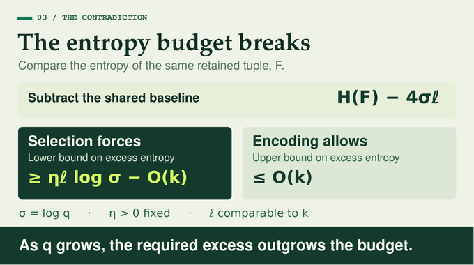
At a successful pivot, the caps bound how many flags the decoder must distinguish. The tree also controls the cost of specifying all the caps. Across each level, the inherited domain costs split between the two children, with a controlled additional cost per successful node. A constant-probability extraction retains a deterministic length comparable to and reduces the combined budget for metadata and slot sizes. A finite number of stages suffices for each fixed . A final marking pass then gives two incompatible estimates for the entropy of the retained tuple .
The terms are bounded by constant multiples of . The excess grows faster because stays comparable to and diverges. Thus some stream avoids a consistent tuple of length .
11. From Prime Fields to the Sharp Exponent
The construction gives vertices and independence number below . Bertrand’s postulate supplies a prime within a constant factor of for every sufficiently large integer . The graph then has no independent set of size . Substituting the scale of into the vertex count gives a lower bound proportional to . Choosing lets the extra logarithmic power absorb the constant, yielding the theorem for all sufficiently large .
The paper leaves open whether a positive constant times is also a lower bound. Exact small values such as are a separate question. The description theorem bounds message length, and the encoder’s search may run through exponentially many proposals. OpenAI’s release announcement gives the publication context, while the Lean scope note records the formalized inequalities and the exponent limit along the natural numbers. The Lean theorem entry point assembles the bounds and the limit.
The sharper Ramsey number bounds show what changed when the proof accounted for the information carried by a selected independent sequence. The geometry rules out five-cliques, and the compression argument makes long independent sequences impossible to guarantee. Explore more Binary Verse AI research on graph coloring and hardness, crossing numbers of complete graphs, and the limits of Weisfeiler–Leman graph refinement. For sampling and formalization, see switch-chain mixing, exact contingency-table sampling, and the Lean formalization of Fermat’s Last Theorem.
What is the Ramsey number r(5,t)?
It is the least number of vertices such that every graph of that size contains either a clique on five vertices or an independent set of size t. A clique has all possible edges among its vertices. An independent set has none.
What did OpenAI’s proof establish about r(5,t)?
It established that r(5,t) grows as t to the fourth divided by the natural logarithm of t raised to the power 3 + o(1). The o(1) term tends to zero as t grows, so the logarithmic exponent is three in the limit. Whether the upper and lower bounds match within a constant factor remains open.
What was the main obstacle in earlier Ramsey number bounds?
The earlier projective lower bound had t to the fourth in the numerator and the sixth power of log t in the denominator. The classical upper bound had the same numerator and the third power of log t in the denominator. The new proof closes the exponent gap by sharpening the analysis of long independent sequences.
Why does the projective-flag graph contain no five-clique?
In a hypothetical five-clique, each of the first four hyperplanes contains the points through its own position and excludes the next point. The five points must then have linearly independent representatives. The fifth hyperplane would have to contain all five vectors in a four-dimensional subspace, a contradiction.
Why is entropy compression essential to the proof?
A long independent sequence selected from the random stream has an entropy surplus above four times the natural logarithm of the field size per flag. The final description permits only that baseline plus a bounded overhead per flag on average. The surplus grows with the field size, giving a contradiction.
Does this proof determine the exact Ramsey number R(5,5)?
No. The theorem describes r(5,t) for large t. The diagonal value R(5,5), also written r(5,5), lies outside the asymptotic calculation.
Does the sharp logarithmic exponent give an exact formula or an efficient construction?
The theorem determines the asymptotic logarithmic exponent. A constant-factor formula remains open. The sparse-pair description theorem bounds message length and gives no general running-time guarantee for its encoding or decoding procedure.