
Two different instructions can draw precisely the same piece of a fractal. With the maps “divide by three,” “divide by three and add one,” and “divide by three and add four-thirds,” nine two-step paths produce only eight affine maps. Counting those paths as separate outcomes gives the construction more information than it actually carries.
OpenAI’s September 24, 2026 preprint proves that the Hausdorff dimension of self-similar measures on the real line is the random-walk entropy rate divided by the Lyapunov exponent, capped at one. The entropy rate uses the combined probabilities of distinct affine compositions. The formula covers exact collisions as well as systems with arbitrarily close distinct compositions, and it applies to unequal contraction ratios of either sign. The precise statement is Theorem 1.1 in the original preprint.
Table of Contents
1. Why Counting Fractal Copies Can Give the Wrong Dimension
When several addresses produce the same map, the resulting piece cannot reveal which address generated it. The exact overlaps conjecture asks whether dimension can still fall below the usual prediction when all finite addresses of the same length give distinct maps. The entropy-rate dimension formula also answers what happens when they collide.
| Feature | What the Paper Establishes |
|---|---|
| Setting | A finite indexed family of similarities on the real line with positive weights. |
| Allowed maps | Unequal or negative contraction ratios, repeated generators, and exact overlaps. |
| Dimension | The map entropy rate divided by the mean logarithmic contraction, capped at one. |
| Formalization | Lean family 148 covers the main formula and two no-overlap consequences. |
A measure assigns weight to the pieces. The attractor records the possible locations regardless of weight. That distinction matters when reading a dimension statement, just as it matters when passing from a set to a measure in the Falconer distance problem.
2. What Are Self-Similar Measures on the Real Line?
Take a finite, nonempty indexed family of affine maps , with real translations and . A negative reverses orientation as it shrinks distances. Choose each symbol independently with probability , with the probabilities summing to one. The resulting limit has a unique Borel probability law , characterized by
Here is the distribution of for of law . The limit comes from applying the compositions to zero, with the earliest symbol outermost. The invariance equation says that one random first map applied to an independent copy of the limit reproduces the original law. The support lies in a bounded interval because the translations are bounded and the contractions are uniformly below one in absolute value.
The paper uses the lower Hausdorff dimension of a measure, the infimum of the Hausdorff dimensions of Borel sets carrying positive mass. Feng and Hu’s exact-dimensionality theorem gives a constant such that for -almost every ,
Here is the ball of radius about . At typical points the mass has exponent as the radius shrinks. In this setting is also the infimum of the dimensions of sets of full measure.
3. Exact Overlaps, Near-Overlaps, and the Loss of Information
For a word , write . An exact overlap is equality of complete maps for distinct words of the same positive length. Both the signed slope and translation must agree. An unequal-length collision also produces a same-length collision by concatenating the words in opposite orders. Invertibility and strict contraction rule out one word being a proper prefix of the other. Equal translations alone can hide a slope difference, and two cylinder images can intersect while their maps remain distinct.
Distinct cylinders can also approach each other faster than any fixed exponential rate without ever coinciding. A grid at one scale can miss a difference that becomes visible on a finer grid. An exact collision erases the distinction at every scale. Earlier separation methods could lose their leverage when the scale needed to distinguish different maps moved too far beyond the nominal contraction depth. Here the proof must track information that can reappear at arbitrarily fine scales.
4. The Entropy-Rate Dimension Formula for Self-Similar Measures
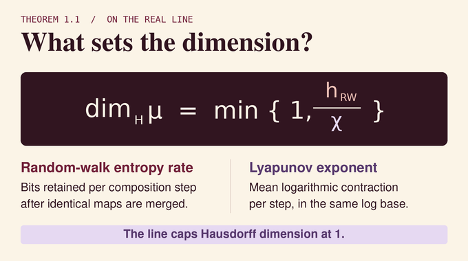
Let , where the are independent symbols with law . A word has probability . The probability of a particular map is the sum of the probabilities of all words of length that give it.
Write for Shannon entropy in bits. A composition of length is a function of two independent block maps, so . Subadditivity gives a limit equal to the infimum of the normalized entropies. The Lyapunov exponent measures the mean loss of logarithmic length per symbol, using absolute slopes.
For every family and positive probability vector in Section 2, Theorem 1.1 gives
The quotient compares bits retained per step with bits of spatial refinement per step. Using the same logarithm base for both quantities leaves the quotient unchanged. The cap comes from the ambient line. The one-symbol entropy measures the address before composing anything. Random-walk entropy measures what the composition retains. For another example of how an entropy result depends on the observed variable, see our coverage of the Courtade–Kumar conjecture.
5. A Worked Example: Nine Symbol Paths but Only Eight Maps
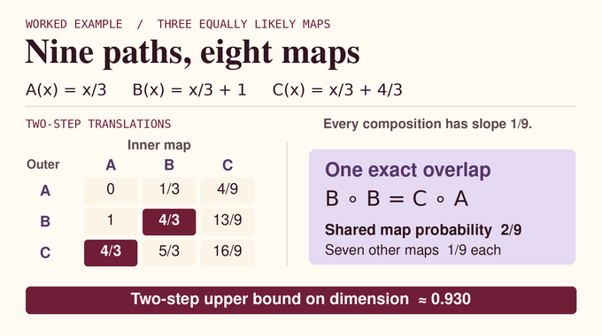
Label the maps , and . In the table, the row map is outermost. Every composition has slope , so the translations alone identify the maps.
| Outer Map | |||
|---|---|---|---|
The repeated translation comes from and . With equal weights, the merged outcome has probability , and the seven others each have probability . The two-step map entropy is therefore bits. Dividing by two gives an upper bound on the entropy rate. Since , the dimension is at most , about 0.930, whereas the symbol formula predicts one. This calculation certifies a dimension drop from a single block length. Computing the exact dimension by the theorem requires the limiting rate.
6. Why Earlier Dimension Theorems Could Not Settle Every Overlap
The Moran–Hutchinson formula gives the similarity dimension of an attractor under the open set condition. This condition allows pieces to touch at boundaries while keeping their open images disjoint. Once separation is removed, those classical results leave open whether near-collisions can cause a dimension drop in self-similar measures even when no two compositions coincide. Bernoulli convolutions supplied an early test case. In their symmetric form, independent fair signs multiply successive powers of a common contraction. Changing the contraction changes the geometry of the random sum.
Hochman showed that falling below the capped symbol formula forces superexponential concentration of cylinder maps. His entropy framework already tracked slopes when ratios differed. That necessary condition left room for actual examples with superexponentially close cylinders and no exact overlaps, constructed by Baker and independently by Bárány and Käenmäki. The preprint discusses both constructions in its historical account.
Arithmetic results covered important classes. Varjú proved full dimension for transcendental Bernoulli convolution parameters in . Rapaport handled the no-overlap formula for algebraic contraction ratios with arbitrary translations, including signed and unequal ratios. Rapaport and Varjú obtained the entropy-rate formula for homogeneous three-map systems with a positive common ratio and rational translations. The new argument works without an arithmetic hypothesis. For related geometric problems, see the Erdős similarity conjecture and the four-dimensional Kakeya conjecture.
7. The First Proof Step: An Upper Bound from Random-Map Entropy
Fix a block length and use distinct composed maps as a new alphabet, with probabilities inherited from . Independent blocks generate the same measure. The new symbol entropy is and its mean contraction depth is . The strong law bounds the number of typical prefixes by their probabilities and bounds the diameters of their cylinder images by their slopes. Summing powers of these diameters yields the dimension upper bound . Taking the infimum over gives .
For the reverse inequality the paper assumes that both and . The first leaves room for entropy gains. The second gives a surplus of map information at typical spatial scales.
8. Uniform Nonsaturation: Why Fair Pairs Create Entropy
Lemma 2.1 defines by averaging the Shannon entropy of the cell label over a uniform grid shift in . Put . For integer , the shifted grids can be nested, so the difference is the conditional entropy of the fine cell given the coarse cell and the shift. It is concave in the law, lies between zero and , and cannot decrease upon adding independent noise.
Lemma 2.2 bounds the fine-grid entropy by for a compactly supported exact-dimensional law. Lemma 2.3 strengthens this asymptotic control for the self-similar measure. If the one-bit deficit approached zero, the smoothed law and its translate by would become almost indistinguishable in total variation. Mixing finitely many consecutive translates would then give near-maximal entropy across a wider scale interval. Stopping the coding at the first prefix below a chosen contraction threshold transfers that bound to all smaller scales, with bounded loss. Telescoping would force an entropy exponent above . Thus uniformly in .
Lemma 2.4 turns that deficit into gain. If is an independent fair bit and , then
A grid much finer than retains information about the shift that a grid much coarser than rarely detects. The same inequality applies to any equal-weight pair at distance .
9. The Finite-Law Pair Bound: Finding Hidden Information at Arbitrarily Fine Scales
For a finite law with support , let be the maximum mass that can be assigned to fair pairs at distances in . Each pair draws half its weight from each endpoint, and all draws at an atom must fit its probability. Capacities are computed separately for each distance band.
Lemma 3.2 bounds times the entropy hidden inside cells of width . The bound is plus a constant depending only on times the sum of capacities over bands with . Here consists of sums of points of . Revealing the sum of independent samples costs at most the sumset term. Randomly perturbing the cuts in successive nested refinements bounds the remaining uncertainty through pairs drawn inside each parent cell. A short displacement is unlikely to cross a random cut. Averaging over cuts charges a pair in proportion to its separation relative to the current cell scale. These charges sum geometrically across the refinement levels. The argument eventually distinguishes every atom, but the depth needed to do so drops out of the bound. A two-atom law makes capacity concrete. If the atoms have weights and , the capacity in their distance band is , since the smaller atom limits the amount that can be matched.
10. Conditioning on Block Types: Keeping Entropy Despite Exact Collisions
Group the symbols into blocks of length . A type records each symbol’s count, so it fixes the product of signed slopes even when the block can be ordered in several ways. Given the types of blocks, the total slope is fixed, and the translation identifies the full composed map. Exact collisions are already merged in its conditional law.
For symbols, recording the types costs at most bits. The map entropy is at least . The type cost per symbol tends to zero as grows. Meanwhile the conditional translation law’s grid entropy is bounded on average by that of plus one bit. With , these estimates leave a surplus proportional to at a grid finer than the typical contraction scale.
The conditional translation is a sum of scaled block digits with fixed scaling factors. Sums of copies can be counted by digit multiplicities at each block, so the logarithm of the sumset grows only as for fixed . The hidden entropy term grows linearly in . Choosing large in Lemma 3.2 forces expected fair-pair capacity proportional to in a finite band of depths, even after restricting to typical contractions.
11. Disjoint Entropy-Gain Windows: The Contradiction That Completes the Proof
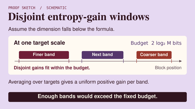
Fix a target depth and examine the entropy of the suffix law between a fine and a coarse grid around that scale. As blocks are removed from the front, this entropy cannot increase. In the paper the target has physical scale , and the two grid widths are and for a fixed large integer . The ratio makes the grids nest, giving an entropy budget of bits. A retained block segment contributes a gain when its scaled pair distances match the target. The proof conditions only on the types through the end of that segment. Averaging the unobserved future gives a signed, scaled copy of . Convexity of the one-bit deficit then transfers its positive lower bound to the average gain.
The paper chooses each new block length after the previous bands’ finite upper endpoints are known. The gap ensures that at any fixed target a window associated with a finer pair band ends before a retained window from a coarser band begins. The disjoint gains telescope inside the entropy budget at that target. Averaging over targets recovers every band’s pair mass. Longer blocks yield fewer candidate starts in inverse proportion to their length, so each band supplies the same positive lower bound on average. Arbitrarily many bands would exceed the fixed budget. The assumed deficit is therefore impossible.
12. Consequences, Lean Verification, and Limits of the Proof
Without exact overlaps, each word gives a distinct map, so . For the attractor under that same hypothesis, , where . Choosing supplies the lower bound through the measure formula, and the cylinder cover supplies the upper bound. For a common positive ratio , the no-overlap measure formula uses . It applies to every positive weight vector for the three maps , and whenever they have no exact overlaps.
The main theorem, the homogeneous positive-ratio no-overlap formula and the no-overlap attractor formula are listed in the family 148 Lean scope notes. The broader OpenAI mathematics release also makes the formal argument available as Lean proof source. For more on formalization in research, see our coverage of Fermat’s Last Theorem and the Navier–Stokes problem.
Dimension one alone gives no density. The preprint also leaves effective separation and a quantitative rate for the entropy limit outside its conclusions. Its result for self-similar measures is precise about what survives at small scales. Exact coincidences are merged before the entropy is measured. Arbitrarily close distinct maps can delay where their information appears, while the formula shows that their proximity causes no further dimension loss. Follow Binary Verse AI for more research explainers, including the entropy conjecture in dynamics, Thorp shuffle mixing, and switch chain mixing.
What is a self-similar measure?
A self-similar measure is a probability distribution preserved by a weighted collection of contracting maps. On the real line, it satisfies .
Why can the standard fractal dimension formula fail when pieces overlap?
Different symbol paths can produce identical affine maps, so counting paths can overstate how much information survives composition. The entropy-rate formula instead uses the combined probabilities of distinct composed maps.
Can self-similar measures lose dimension without exact overlaps?
Without exact overlaps, the theorem gives the usual symbol entropy divided by the Lyapunov exponent, capped at one. Superexponentially close but distinct cylinder maps cause no additional dimension drop.
What is the difference between random-walk entropy and the Lyapunov exponent?
The random-walk entropy rate measures the information retained in the composed map per step. The Lyapunov exponent measures the average logarithmic contraction per step. Their ratio gives the Hausdorff dimension, capped at one.
Does the entropy-rate dimension formula allow negative and unequal contraction ratios?
Yes. The theorem allows finite nonempty families of nonzero real contraction ratios of absolute value below one, with strictly positive weights. This includes orientation-reversing maps, unequal ratios and repeated generators.
Does Hausdorff dimension one mean a self-similar measure is absolutely continuous?
Full Hausdorff dimension alone does not imply absolute continuity or guarantee a density. The theorem gives a dimension formula.
Does OpenAI’s proof extend the entropy-rate dimension formula to higher dimensions?
The theorem applies to the real line. The general higher-dimensional formula lies outside its scope.