
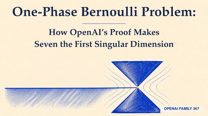
A free boundary can look perfectly smooth in low dimensions yet develop a singular cone when enough coordinates are available. The one phase Bernoulli problem now has an exact threshold: the September 24, 2026 OpenAI mathematical manuscript proves that every nonzero one-homogeneous global minimizer is a half-space solution through dimension six. A nonflat minimizing cone already known in dimension seven makes the threshold sharp. Consequently, interior free boundaries of local minimizers are smooth through dimension six, while higher-dimensional singular sets obey a sharp codimension-seven bound. The crucial advance is not a newly discovered cone, but a Hessian-sensitive instability argument that rules out the last two unresolved dimensions.
Table of Contents
1. What Did OpenAI’s Proof Establish About the One-Phase Bernoulli Problem?
The paper’s Theorem 1.1 identifies the first dimension that admits a nonzero, nonflat, one-homogeneous global energy minimizer. Its Corollary 1.2 transfers that classification to interior free-boundary regularity. The result applies to the constant-coefficient Alt–Caffarelli energy with unrestricted admissible Sobolev competitors, not to every equation called a Bernoulli problem.
| Setting | Established conclusion |
|---|---|
| Dimensions 1–6 | Every nonzero one-homogeneous global minimizer is flat; local minimizers have smooth interior free boundaries. |
| Dimension 7 | A nonflat global minimizing cone exists; singular points of a local minimizer are locally finite. |
| Dimensions 8 and above | The singular set has Hausdorff dimension at most n − 7, and the bound is attainable. |
The October 2026 research release includes the manuscript among OpenAI’s mathematical results. The paper gives the analytic proof; neither the announcement nor the associated Lean comparator should be mistaken for an independently completed formal verification of the entire theorem.
2. The Alt–Caffarelli Functional: What Energy Does the Problem Minimize?
Let be a ball and let be a Sobolev function. The one-phase Bernoulli free boundary problem minimizes the sum of Dirichlet energy and the volume occupied by the positive phase:
The indicator equals one where the function is positive and zero otherwise. For a global minimizer, the comparison must hold on every ball against every nonnegative with the same boundary trace, expressed by . A local minimizer satisfies the same comparison on balls compactly inside its domain. This is stronger than merely being stationary against a restricted family of perturbations.
Within the positive phase, variations preserve its volume and yield the harmonic equation. At a smooth interface, moving the boundary balances energy against the volume penalty:
The boundary gradient points toward the positive side. This variational balance is distinct from the fully nonlinear setting discussed in our infinity-Laplacian regularity analysis, although both concern delicate PDE regularity.
3. A Worked Half-Space Example: What Makes a Bernoulli Minimizer Flat?
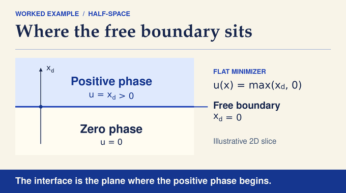
Choose a unit vector and measure position along that direction. The basic minimizer rises linearly on one side and vanishes on the other:
For , the positivity region is , the zero region is , and their common boundary is the plane . In the positive half-space the gradient has unit length and the Laplacian vanishes. In any small ball centered on the interface, the boundary cost and gradient cost sit at the Bernoulli equilibrium. The global minimizing property is a standard comparison result, not implied by these two first-order checks alone.
A nonflat minimizing cone is fundamentally different: rescaling preserves its shape, but the interface is not a hyperplane. Its vertex is a candidate singularity that no rotation can remove.
4. Blowups and One-Homogeneous Minimizers: How Are Singularities Detected?
To inspect an interior free-boundary point , magnify the minimizer while dividing its height by the same scale. Along a sequence of shrinking radii, the rescalings have subsequential limits:
The paper collects the needed compactness, nondegeneracy, and regularity inputs in Proposition 2.1. Every blowup is a nonzero one-homogeneous global minimizer. A point is regular when at least one blowup is flat, because improvement-of-flatness results then turn that asymptotic picture into a smooth local interface. A point is singular when no blowup is flat.
Homogeneity means for positive scales. Thus the critical question is not whether arbitrary PDE solutions can have complicated interfaces, but whether a genuinely nonflat cone can win the full energy comparison. This use of rescaling and classification also appears, under different hypotheses, in geometric PDE questions such as the dimension-eight De Giorgi problem.
5. Why the Critical Dimension Was Previously Trapped Between Five and Seven
The classification was not open in every dimension. Caffarelli, Jerison, and Kenig established a low-dimensional stable-cone rigidity result, extended by Jerison and Savin to smooth-link stable homogeneous solutions through dimension four. This gave a lower bound for the first possible nonflat minimizing cone. De Silva and Jerison then constructed a genuine nonflat one-homogeneous global minimizer in seven dimensions, producing an upper bound.
| Dimension | Status before the 2026 proof | Status after |
|---|---|---|
| 1–4 | Flatness known for minimizing cones | Unchanged |
| 5–6 | No complete exclusion of nonflat minimizing cones | Nonflat minimizers excluded |
| 7 | De Silva–Jerison minimizing example existed | First possible singular dimension confirmed |
The new manuscript closes those two cases without imposing symmetry on the minimizing cone. It does not claim to invent the De Silva–Jerison cone or classify all stationary configurations. The distinction between energy minimizers and merely stable solutions matters throughout the argument.
6. Why the Earlier Hessian Stability Tests Failed
For a homogeneous harmonic function, the Hessian measures deviation from linearity. Flat solutions have vanishing Hessian throughout their positive phase, whereas a nonflat component has nonzero Hessian somewhere. Earlier work tested stability using powers of its norm. But the interior differential estimate and the curvature term at the boundary demand competing restrictions on those powers; one cannot simply pick a universal exponent that makes both inequalities work in dimensions five and six.
Jerison and Savin already improved the four-dimensional argument by using more refined eigenvalue information. OpenAI’s manuscript pushes this idea further: it retains the normalized tensor shape, its interaction with the spherical gradient, and a separate divergence-carrying vector field. The test and flux are designed together rather than patched together after separate estimates.
The result is an actual strict remainder, not merely an inequality at equality. This is why the method resembles, only at the level of analytical strategy, other delicate elliptic estimates such as those in our Lane–Emden conjecture explainer. The mathematical claims in this article remain specific to Bernoulli minimizers.
7. Dimension Reduction and Suspension: Bringing Both Cases onto the Five-Sphere
Assume for contradiction that the smallest dimension carrying a nonflat minimizing cone is five or six. At a nonvertex free-boundary point, a blowup is invariant along the direction from the origin. Removing that invariant coordinate produces a lower-dimensional global minimizer, which must be flat by minimality of the chosen dimension. Regularity then makes every nonvertex boundary point smooth.
Intersect the positive cone with the unit sphere. Its spherical link has finitely many smooth components with disjoint closures. Select a component on which the spherical Hessian is not identically zero. A six-dimensional cone already gives a working link on . A five-dimensional cone can be extended constantly along one additional Euclidean coordinate without losing global minimality. This operation is called suspension.
The suspended link has a smooth side and two exceptional tips, one at each endpoint of . Those tips cannot be treated as regular boundaries. Their removal later requires a separate integrability argument. The payoff is that both hypothetical dimensions now share the same spherical dimension, and therefore the same sharp stability constant.
8. Spherical Hessian Geometry and the Stability Inequality
Write the homogeneous cone as on the unit sphere. On a positive component of , set . The trace-free spherical tensor and its norm encode the Euclidean Hessian transverse to the radial direction:
Here denotes the spherical identity tensor. The paper derives Codazzi symmetry, , and a Bochner identity. The latter produces a positive square of the third derivatives, which becomes the key weight for controlling zeros of .
On a smooth side boundary the inward unit normal is , and the curvature sum is . For the selected nonflat component, the paper proves . The second variation of the full minimizing energy, followed by a sharp radial Hardy calculation, gives the spherical stability constraint:
The coefficient four is the squared Hardy threshold for the five-dimensional spherical link; it is not an adjustable constant. Spherical geometry is also central, for different reasons, in our hot spots conjecture coverage.
9. The New Scalar Test and Vector Flux: How the Proof Creates a Strict Stability Gap
On the region where , normalize the Hessian and its first derivative by and . The coefficient functions depend on these normalized tensors, the spherical function , and its gradient . This retains orientation and eigenvalue information discarded by the plain test .
The authors construct rational tensor polynomials , , , and , with , and fix the exponent . Their scalar test and companion vector flux are:
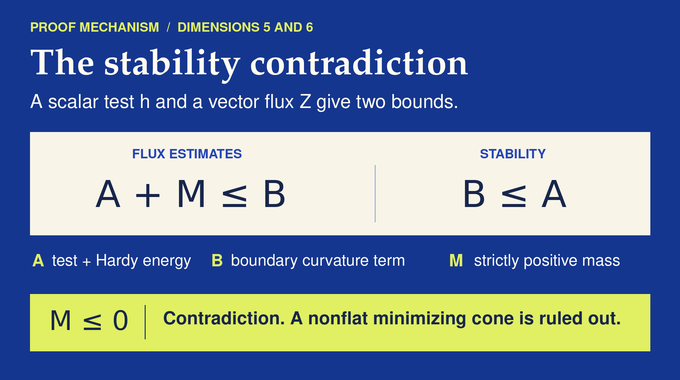
The core advance is a matched pair of inequalities. The interior divergence exceeds both the test energy and the Hardy term by a strictly positive mass; the inward boundary flux has the sign needed to compare with curvature. With , the paper proves:
Integrating both estimates and applying stability would force a positive quantity to be nonpositive. The remaining obstacle is to justify that integration where the Hessian vanishes and, in the suspended case, at the two tips.
10. Exact Tensor Certificates: How Are the Interior and Boundary Inequalities Verified?
The finite algebraic certificate is the longest technical component of the paper. Its variables are a normalized trace-free five-by-five matrix, a symmetric trace-free three-tensor, and the relevant scalar and vector data. The derivative of the flux appears to contain uncontrolled fourth derivatives of the original function. A Laplacian contraction and an antisymmetric curvature contraction remove them, leaving tensor expressions that can be certified pointwise.
At a regular boundary, reflection across the normal direction removes the components of the third derivative that the Bernoulli condition does not determine. What remains is an inequality involving four tangential eigenvalues. Instead of sampling those configurations numerically, the authors use rational polynomials, weighted tensor squares and explicit coefficient bounds.
The manuscript reports 19 Gram comparison blocks, 1,714 nonzero collected interior graph keys, and an 11-coefficient boundary remainder. The arithmetic uses the common denominator and exact integer comparisons. Its quoted positive margins include and . These constants are certificates for inequalities, not observed performance metrics.
This is finite symbolic verification inside a much larger analytic proof, not a declaration that every step is Lean-certified. The supplied Lean scope note explicitly limits its linked statement to the dimension-seven existence side. Moreover, the supplied comparator theorem file currently ends with `sorry`, indicating an unfilled proof placeholder. Related discussions of rigorous PDE arguments appear in our Calderón inverse problem explainer, but they do not validate this certificate.
11. Hessian Zeros, Suspension Tips, and the Final Contradiction
The normalized field is undefined wherever . Simply deleting those points would leave an unproved integration step. Section 7 establishes a weighted Bochner estimate on the original smooth spherical component:
The proof regularizes the squared Hessian norm by adding a positive parameter, integrates the Bochner identity against a cutoff, and then lets the parameter vanish. The exponent makes the decisive coefficient positive. Near the suspension tips, the exact metric and measure introduce powers of that remain integrable.
Smooth product cutoffs now exclude both the Hessian-zero set and small neighborhoods of the tips. The divergence theorem, the boundary flux sign, and spherical stability combine to bound a positive bulk integral by three cutoff-error terms. Weighted integrability makes all three errors vanish as the cutoffs are removed.
But the selected component was deliberately chosen so that is not identically zero. Hence its weighted Hessian mass is strictly positive. The mass survives the cutoff limit, contradicting the stability bound. This closes the contradiction in both dimensions five and six.
12. What Dimension Seven Changes: Smoothness, Isolated Singularities, and the Sharp n-7 Bound
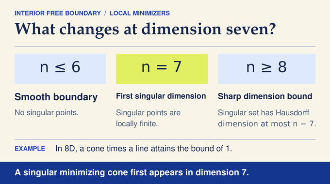
With dimensions five and six excluded, the existing seven-dimensional De Silva–Jerison cone sets the precise threshold. Standard dimension reduction then translates cone rigidity into a statement about every interior free boundary of a local minimizer of this energy. Up to dimension six, the singular set is empty. In dimension seven it is locally finite, so singular points cannot accumulate within a compact subset of the domain.
For larger dimensions, “at most ” means a Hausdorff-dimension bound, not a count of singular points. Sharpness is constructive: take the known seven-dimensional minimizing cone and make it independent of extra coordinates. The product remains globally minimizing, and its singular set contains an -dimensional Euclidean factor.
The smoothness conclusion is powerful but carefully scoped. It concerns interior points of locally minimizing, constant-coefficient one-phase Bernoulli energies. It does not automatically cover arbitrary stationary free boundaries, changed volume penalties, rough coefficients, or all nonlinear interface models. For contrast, our Brennan conjecture article treats different geometric-analytic regularity constraints.
The one-phase Bernoulli problem now has a sharp geometric dividing line: flat minimizing blowups below seven, with genuinely singular minimizing geometry first possible in seven dimensions. The manuscript’s achievement is the stability mechanism that completes that dividing line, while its finite certificates and assumptions remain open to careful mathematical scrutiny. Explore more paper-led analysis at Binary Verse AI, where the aim is to understand the argument rather than repeat the announcement.
What is the formula for the one-phase Bernoulli problem?
The problem minimizes J(u; B) = ∫_B (|∇u|² + 𝟙_{u>0}) dx over admissible Sobolev functions with prescribed boundary values. The gradient term penalizes variations in the function, while the indicator penalizes the volume of the positive region. The interface between the positive and zero regions is the free boundary.
What is an example of a flat one-phase Bernoulli minimizer?
A standard example is u(x) = max{x_d, 0}. It is positive when x_d > 0, vanishes when x_d ≤ 0, and has the flat free boundary x_d = 0. Rotations give the corresponding half-space solutions in other directions.
Why is seven the critical dimension for Bernoulli minimizers?
The paper proves that every nonzero one-homogeneous global minimizer is flat in dimensions one through six, while a nonflat one-homogeneous global minimizer exists in dimension seven. Therefore, seven is the first dimension permitting a singular minimizing cone.
Did OpenAI construct the first seven-dimensional singular Bernoulli minimizer?
No. De Silva and Jerison had already constructed a nonflat seven-dimensional global minimizer. The new proof excludes the previously unresolved dimensions five and six, completing the critical-dimension classification.
Why were dimensions five and six difficult to exclude?
Earlier Hessian-norm stability tests faced incompatible interior and boundary requirements. The paper combines a normalized Hessian-dependent scalar test with a carefully constructed vector flux to produce a strict contradiction with stability.
What does the singular-set bound n-7 mean?
For local minimizers in dimension n ≥ 7, the singular set has Hausdorff dimension at most n − 7. In dimension seven, it is locally finite. Products of the known seven-dimensional minimizing cone with Euclidean space show that the bound is sharp.
Does the result prove that every Bernoulli free boundary is smooth below seven dimensions?
No. The smoothness theorem concerns interior free boundaries of local minimizers of the specified constant-coefficient one-phase Bernoulli energy. It does not automatically apply to arbitrary stationary solutions, nonminimizing configurations, or modified Bernoulli models.