
Suppose a quantum algorithm can query a vast string of bits in superposition, while a classical algorithm has to inspect one bit at a time. How can the classical algorithm know where to look? The November 2026 proof of the Aaronson Ambainis Conjecture gives an answer. Every nonconstant bounded polynomial of low degree on the Boolean cube has a variable whose influence is bounded below by a polynomial in its variance and inverse degree. Since a quantum algorithm’s acceptance probability is such a polynomial, a classical decision tree can query influential bits and approximate that probability on most uniformly random inputs. The guarantee counts input queries. The work done between queries can still be expensive.
Table of Contents
1. What Is the Aaronson Ambainis Conjecture?
Scott Aaronson raised the problem in a 2008 lecture. In their 2014 paper on structure in quantum speedups, Aaronson and Andris Ambainis asked whether a polynomial that stays between zero and one on all bit strings, and has variance at least under the uniform distribution, must have a variable with influence at least , where is the degree. Here the exponent denotes a universal power, independent of how many input bits there are.
| Key Fact | What the Paper Establishes |
|---|---|
| Result | A polynomial lower bound on the influence of some variable in every nonconstant bounded polynomial on the Boolean cube. |
| Main Bound | for a universal positive constant and degree bound . |
| Original Form | An influence of at least for variance at least in the original zero–one convention. |
| Query Consequence | A deterministic classical decision tree can approximate a quantum algorithm’s acceptance probability on most uniform inputs with polynomially many queries. |
| Proof Status | David Turturean’s November 2026 preprint and a public Lean 4 formalization of the theorem and corollary. |
The dimension-free requirement matters. If an output depends a little on each of a million bits, a bound that shrinks with the input length gives the classical algorithm little guidance. Boundedness and degree together prevent that influence from spreading arbitrarily thin at fixed variance. The influential coordinate can change after an answer fixes one bit. That is what makes the resulting decision tree adaptive.
2. Why Quantum Query Complexity Leads to Low-Degree Polynomials
The polynomial comes from how an oracle call changes a quantum state. In the bit-query model, a query to an input position routes an amplitude according to whether that bit is zero or one. The new amplitudes are therefore linear combinations of the old ones with coefficients affine in input bits. Input-independent operations mix amplitudes without increasing their degree. After queries, every amplitude has degree at most .
The algorithm’s acceptance probability adds squared magnitudes of the accepting amplitudes. This doubles the degree bound to . On the bit cube, positive powers of a bit can be replaced by that bit, so the probability has a real multilinear representation. It is between zero and one even if it takes many intermediate values. That range is why a result only about Boolean-valued functions would leave the simulation question open. Our coverage of quantum query complexity provides another example of how much depends on the precise oracle task.
3. Variance, Influence, and a Worked Example on the Boolean Cube
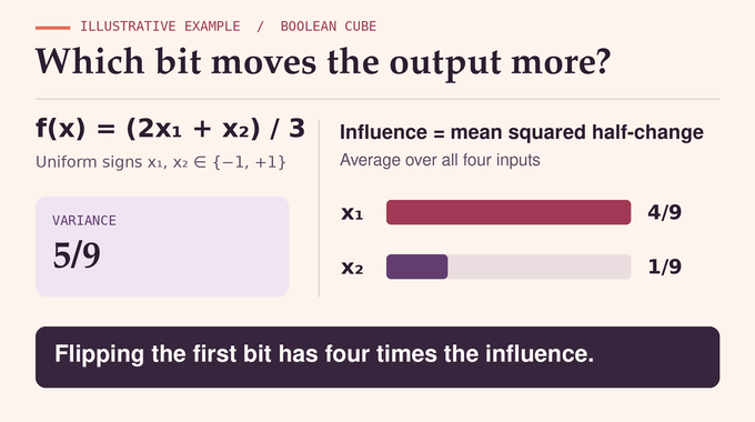
Write for the sign cube and take uniformly from it. The manuscript uses for the point obtained by flipping coordinate , and for flipping all coordinates in a set . Variance is the mean squared deviation from the mean. The degree is the largest number of distinct coordinates multiplied together in any term of the unique multilinear expansion with a nonzero coefficient. The influence of a variable uses the squared half-change under a flip.
For a worked example, take . Its four values lie in the required range, its degree is one, and its mean is zero. Since the two signs are independent, the cross term averages to zero. Flipping the first sign gives a half-change of . Flipping the second gives . Therefore , while and . Any unused coordinates have zero influence. The example shows how the mean squared flip distinguishes the two relevant bits even though both flips always change the output. For related uses of the Boolean cube, see our coverage of the Courtade–Kumar conjecture and the quadratic sensitivity conjecture.
4. Why Earlier Approaches Could Not Prove the Conjecture
Earlier general results could guarantee a coordinate of influence at least in the original bit convention. At fixed variance, that guarantee decays exponentially with degree. Polynomial dependence was known for Boolean-valued functions and for special real-valued cases, including certain multilinear forms with equal-magnitude coefficients. A 2019 proof attempt by Nathan Keller and Ohad Klein was later withdrawn.
Lovett and Zhang’s work on fractional certificates came closer. Their strategy would succeed given a conjectured inequality about the distance from one set of cube vertices to the convex hull of another. Turturean’s manuscript gives a counterexample to that inequality as stated for arbitrary sets, using tribes, a Boolean function that takes the OR of many disjoint AND blocks. The new proof keeps the idea of examining where a real-valued polynomial crosses a threshold. It replaces the convex-hull step with an inequality that uses certificates from both sides of the threshold. This lets the proof combine information across all thresholds, including those at which relatively few vertices change sides.
5. The New Theorem on Variable Influence
Theorem 1.1 applies to with integers and and degree at most . Some coordinate satisfies the following bound.
At fixed variance, the degree appears to the sixth power in the denominator. At fixed degree, the variance appears to the five-halves power. The leading constant is about . Constant functions have zero variance, so the lower bound is informative when the output varies.
Corollary 1.2 returns to the original bit cube. For a real polynomial of degree at most with values in on and variance at least , the original influence is the mean squared full change when bit flips. For some bit it satisfies the following chain.
Changing variables via and setting multiplies variance by four and makes the sign-cube half-change equal to the original full change. The last inequality absorbs the constant into a convenient exponent, using the fact that the variance of a probability is at most one quarter.
6. How the Determinant Argument Produces a Controlled Bijection
Start with a Boolean function and let contain its one-valued vertices. A wing at is a set of coordinates such that every subset of them can be flipped from while staying in . Choose one wing per vertex. Theorem 3.1 produces a permutation of that changes every wing coordinate at each vertex. For any coordinate , it also bounds how many times and agree there, by , the number of edges in direction crossing from one to zero, counted once per edge. This simultaneous control strengthens the existence statement equivalent to Reimer’s Butterfly Lemma.
The agreement matrix has one row and column per vertex in . Its entry is the product of formal variables over coordinates where and agree. A permutation in the determinant expansion contributes a monomial whose exponent of counts its agreements in coordinate . Factoring out contributions from edges that stay inside bounds those exponents in the lowest-total-degree monomials by the crossing-edge counts. Signed combinations of rows along each wing then cancel entries that agree on any wing coordinate. The transformations preserve the lowest-degree part of the determinant, so a surviving monomial supplies a permutation satisfying both constraints. For a different use of determinants in complexity theory, see the permanent versus determinant problem.
7. From Antipodal Pairs to the All-Pairs Inequality
A fractional certificate for a Boolean output at a vertex assigns nonnegative weights to coordinates. Any set of flips that changes the output must collect at least one unit of weight. At opposite vertices with different outputs, the two certificates identify a wing whose coordinates can be flipped safely from the one-valued endpoint. The determinant bound then controls the cost of getting back to the one-set from the zero-valued endpoint using coordinates outside that wing.
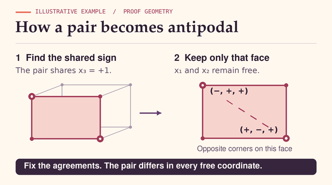
To compare any two vertices and with different outputs, fix the coordinates on which they agree and leave the others free. The pair is antipodal in exactly this subcube. For a chosen set of free coordinates, each crossing edge in one of those directions appears in exactly one restriction. Each direction is free in choices of coordinate sets, so adding over all restrictions gives Proposition 5.2. With the zero-set, the certificate weight at , and auxiliary weights, it reads as follows.
8. Fractional Certificates, Chebyshev Bounds, and Linear Programming
For a real-valued , the manuscript calls a certificate a row. A row at assigns enough weight to each flipped set to cover the absolute output change . The sum of its coordinate weights is its cost. Theorem 6.8 gives a row at every point with cost at most . We use to denote a common upper bound on the chosen row costs.
The dual problem assigns nonnegative weights to blocks of flips, with at most one unit of weight passing through any coordinate. Maximizing the weighted sum of absolute changes gives twice the fractional block sensitivity in the normalization cited by the paper. The proof uses Chebyshev polynomials to encode overlapping blocks as single flips in new variables. Markov’s endpoint derivative inequality then controls the sum of these flips through the degree. Linear programming duality turns the packing bound into a row at each point. Agarwal and Ben-David had already established a sharper row bound with half that coefficient. The proof in the manuscript derives the looser constant directly. It also bounds the sum of single-bit absolute changes at any point by , so the sum of their means has the same bound. This polynomial use of boundedness has a different objective from the extremal construction in our Littlewood polynomials coverage.
9. Integrating Level Sets and Averaging Coordinates to Finish the Proof
At each threshold , set . Away from equality, dividing the row at by gives a fractional certificate for this Boolean function. Crossing the threshold takes at least that much change. For a pair with , the all-pairs inequality then carries the product of distances from the threshold. Its integral is cubic.
On the edge-count side, an edge crosses the threshold over an interval whose length is its absolute increment. Write and . Keeping pairs across a cut at and removing the auxiliary weights using Cauchy–Schwarz gives Theorem 7.6. In its upper-tail form, it bounds the third moment above the cut, multiplied by the mass on the other side, by . The lower-tail form follows by replacing the function with its negative. Applying it at a median to both and bounds by . The third moment is at least .
To get squared influence, average out coordinates whose squared influence is too small relative to their mean absolute increment. Their summed influence is at most two fifths of the variance, so at least three fifths of the variance survives, and the row bound survives by averaging. The coordinate with a large mean increment in the averaged function was kept, so its squared influence in the original function also has a lower bound. The denominator in that bound is proportional to . Substituting the two degree bounds yields . The extra variance factor in the averaging step turns the exponent into .
10. What the Proof Establishes About Quantum Speedups
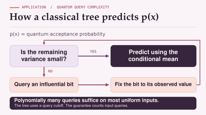
To approximate a -query quantum algorithm’s acceptance probability, the deterministic classical tree queries an influential bit and restricts the polynomial to the observed value. Once the conditional variance is at most , it returns the conditional mean. Chebyshev’s probability inequality controls the error at such leaves. Under a uniform restriction, the expected total influence of the remaining polynomial drops by the influence of the queried bit. Before stopping, each such drop is at least by Corollary 1.2. This budget bounds the expected number of queries, and a fixed cutoff adds at most another to the exceptional fraction. Section 1.3 gives the following bound on the query count.
The approximation is within additive error on at least a fraction of the uniform inputs. A dense promise retains a useful guarantee when the exceptional fraction is chosen small relative to the promise density. A rare promise can lie inside the exceptional set. In Shor’s period-finding setting, the oracle has periodic structure, so the uniform-input guarantee leaves that source of speedup intact. See our coverage of exact quantum factoring for a separate result about factoring. The decision tree’s bound also leaves open the computational cost of finding its next bit and evaluating a conditional mean. Gate counts and circuit lower bounds measure other resources, as our coverage of quantum circuit lower bounds illustrates.
11. Lean Verification, Proof Limitations, and Remaining Open Problems
Physical Superintelligence’s November 6 announcement credits an internal research system running instances of a nonpublic Anthropic model. David Turturean developed the harness, reviewed the manuscript and takes responsibility for it. The public Lean 4 repository documents kernel checks for the main theorem and original-normalization corollary. Its scope notes list the quantum consequences in Section 1.3 and the open questions in Section 9 among the passages without a formal counterpart. For another example of formalization, see our coverage of Fermat’s Last Theorem in Lean.
The paper asks if the variance exponent can drop from to . The average of independent signs has degree one, variance , and every influence equal to , so an exponent below two cannot work uniformly. The optimal degree exponent is also open. The best universal coefficient in the quadratic row-cost bound lies between and , and a direct combinatorial construction of the controlled bijection remains open.
The Aaronson Ambainis Conjecture proof makes a concrete link between variance and the next bit a classical decision tree can read. Follow Binary Verse AI for more research explainers on what different models of computation can prove about their limits.
1. Has the Aaronson–Ambainis conjecture been proved?
Yes. The November 2026 paper proves that every nonconstant bounded low-degree polynomial on the Boolean cube has a variable with influence bounded below by a polynomial expression in its variance and inverse degree. The main result has also been formalized in Lean 4.
2. Why was the Aaronson–Ambainis conjecture difficult to prove?
Earlier general influence bounds decayed exponentially with polynomial degree. The new proof establishes a determinant-based all-pairs inequality in place of a conjectured inequality that fails for general sets, then integrates across the polynomial’s level sets.
3. Does the proof rule out exponential quantum speedups?
For approximating a quantum algorithm’s acceptance probability on most uniformly random inputs, the proof guarantees a deterministic classical algorithm with a query count polynomial in the quantum query count and the inverse error parameters. It leaves open exponential advantages in running time and on suitably structured inputs.
4. Why does the proof not invalidate Shor’s algorithm?
Shor’s period-finding subroutine works with structured periodic functions. The conjecture’s simulation guarantee allows an exceptional fraction of unrestricted inputs, which can include a rare promise such as periodic structure.
5. How does an influential variable allow classical simulation?
A classical decision tree queries an influential bit and restricts the acceptance-probability polynomial to the observed value. It repeats until the conditional variance is small enough to predict the probability by the conditional mean, subject to a query cutoff that controls the exceptional fraction.
6. What mathematical questions remain open after the proof?
The optimal dependence on variance and degree remains unknown. The paper asks whether the variance exponent can improve from five halves to two.