
Euler’s totient function sends both 8 and 12 to 4. Computing either output is easy. Counting every distinct output, without counting 4 twice, leads to a question that has resisted precise asymptotics for decades. OpenAI’s September 25, 2026 manuscript gives an asymptotic formula for the number of totients, together with the Erdős–Hall scaling result: multiplying a sufficiently large cutoff by any fixed positive factor multiplies the count asymptotically by that factor.
The coefficient is not a newly discovered decimal constant. It retains arithmetic information through a convergent construction. The research manuscript explains how prime-factor geometry and careful duplicate removal produce that coefficient. Released through OpenAI’s mathematics initiative, this is a number-theoretic proof, not a measured improvement in a factoring program.
Table of Contents
1. What Is the Number of Totients, and What Does V(x) Count?
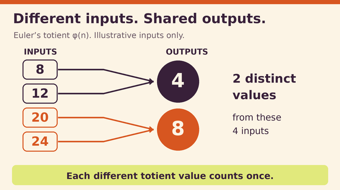
Euler’s totient counts integers from 1 through that are coprime to , meaning their greatest common divisor with is one. For 8, these are 1, 3, 5, and 7. Thus .
The totient counting function records the range of this arithmetic function:
Here means the number of elements, and inputs are positive integers. The cutoff bounds the output, not its preimage. Simply evaluating inputs up to need not find every output below .
| Topic | What It Means |
|---|---|
| Counted object | Distinct positive outputs of Euler’s totient function, each counted once. |
| Duplicate example | : two preimages contribute one output. |
| Main advance | An asymptotic equivalent and fixed-dilation limits for every fixed positive multiplier. |
| Coefficient | A positive, bounded phase-dependent function, defined independently of the count. |
| Practical scope | A theorem about eventual growth, without a tested fast enumeration algorithm. |
The same distinction between representations and outputs appears in our inverse Goldbach explainer: several input pairs can generate one integer. A counting argument must decide which object receives the tick mark.
2. The Original Counting Problem: What Erdős and Hall Wanted to Know
Totient values have natural density zero: . Their share of the positive integers eventually vanishes. This does not mean there are only finitely many. Every prime supplies the distinct totient , already giving roughly values up to .
In 1976, Erdős and Hall asked whether for fixed . Does doubling a large interval approximately double its supply of totients, despite their thinning density? That is compatible with zero density, just as the prime count has nearly linear growth over fixed multiplicative changes while primes become proportionally rarer.
As our Artin primitive-root analysis also illustrates, infinitude, density, and a precise growth law are different conclusions. Here the new limit specifies behavior across fixed multiplicative intervals.
Erdős Problem 416 brings together this scaling question and the search for an asymptotic formula. These concern distinct totient values, not an algorithm for evaluating one totient. Our short Egyptian fractions article covers another Erdős question where the exact quantitative target matters.
3. What Earlier Mathematics Established, and Why Ford’s Estimate Wasn’t Enough
The distribution of totients became progressively clearer through work by Pillai, Erdős, Erdős–Hall, Pomerance, and Maier–Pomerance. The progression concerns increasingly precise population estimates.
| Topic | What It Means |
|---|---|
| Pillai, 1929 | Established that totient values occupy a vanishing proportion of integers. |
| Erdős, 1935 | Sharpened the upper bound to almost the reciprocal-logarithmic scale. |
| Erdős–Hall, 1976 | Strengthened lower bounds and posed the fixed-dilation question. |
| Maier–Pomerance, 1988 | Determined the leading constant in the squared triple-logarithmic exponent. |
| Ford, 1998 | Determined the order up to bounded multiplicative uncertainty, with structural estimates for typical preimages. |
Ford’s 1998 distribution theorem, using its revised 2013 version, gives the following expression. All logarithms are natural, and means applying the logarithm times.
The constants are and . The notation denotes a bounded quantity. Exponentiating it leaves a bounded multiplicative factor, which need not approach one or cancel between endpoints.
An asymptotic equivalent is stronger: the true count divided by its proposed main term tends to one. The difference resembles the distinction between frequency and isolated examples in large prime gaps. More detail about abundance can answer a different mathematical question.
4. OpenAI’s Asymptotic Formula: Theorem 2.1 Explained
The new asymptotic formula for the number of totients is:
The symbol means ratio tending to one as . To define the scale, first set for . These positive coefficients determine the unique root satisfying:
Set and . This is not Euler’s constant. The recurrence starts with :
For sufficiently large , the remaining definitions are:
The auxiliary only abbreviates the displayed quotient. Thus is its fractional part, and empty products give . The earlier constants satisfy and .
The coefficient is bounded above and bounded away from zero uniformly in phase. Its first argument is the constant weight one. “Explicit” means independently defined arithmetic approximations, not an elementary closed form or a ready numerical calculator.
5. The Prime-Factor Decomposition Behind the Proof
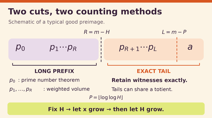
Order the prime factors of a typical preimage from largest to smallest and write:
Two cuts separate the parts: and , where . The parameter is fixed while tends to infinity, then allowed to grow. Reversing those limits would invalidate the finite-tail argument.
Count by the prime number theorem.
Replace weighted prime sums by volume.
Cut at R: keep the later factors discrete
and
Combine witnesses with the same totient.
The long prefix ends at . Its primes become large enough for continuous approximations. The remaining primes and smooth cofactor form the arithmetic tail. “Smooth” means all prime divisors lie below a specified bound.
For fixed , the tail is bounded independently of . Ford’s structure estimates discard a small exceptional collection of values. Crucially, outside that collection, every preimage has the required structure. Finding only one convenient preimage would not later justify conclusions about the least one.
Prime-factor organization also drives our Erdős–Pomerance explainer, although its target is a joint distribution for consecutive integers rather than the range of the totient function.
6. How Simplex Geometry Turns Prime Factors Into a Counting Formula
The useful coordinates are , with . They compress enormously separated prime sizes into a manageable geometric region. Weighted inequalities constrain later coordinates relative to earlier ones.
For the true simplex in coordinates, define nonnegative slacks . A slack measures room left in an inequality. The recurrence gives:
After rescaling to , the slacks are nonnegative and sum to one. This is a standard simplex, whose original-coordinate volume is precisely .
Prime sums become volumes because reciprocal shifted-prime weights, , have approximately unit mass in suitable unit boxes of double-logarithmic coordinates. Mertens’ theorem supplies that conversion. Concentration bounds show that boundary strips and unusually positioned coordinates contribute little.
Smooth-cofactor estimates then control the residual integer rather than silently discarding it. The normalized triangle makes the role of a slack concrete: moving toward its diagonal consumes the residual coordinate, while crossing the diagonal would make that coordinate negative and therefore inadmissible.
The resulting volume counts weighted prime configurations. It still needs an arithmetic argument to count distinct outputs. As in our complete-graph crossing-number explainer, geometry is an intermediate language whose connection to the original counting target must be justified.
7. The Shifted-Prime Sieve: Why Different Prefixes Rarely Produce the Same Totient
Distinct prefixes might yield the same product of shifted primes. For a good representation with tail totient , the value is:
Compare two representations and cancel their common prefix. At the first unequal prime, the remaining equality constrains two products of shifted primes. The proof aligns their large factors and compares them in layers.
Each sieve application involves only two or three linear forms, even though the number of layers grows. Upper bounds limit how often the simultaneous primality requirements can occur. The argument also accounts for recovering hidden tuple data from residual factors.
This last bookkeeping matters: bounding the number of collision values alone is insufficient if one value supports many tuples. The paper bounds ordered pairs of distinct tuples with the same output, on a scale negligible relative to the main count after the prescribed limits.
Consequently, almost every counted value has a unique long prefix. This does not imply a unique complete preimage. Nor does the sieve assume independent primality. Readers of our two-point Chowla explainer will recognize why arithmetic dependence needs a proof rather than a probabilistic slogan.
8. Counting Arithmetic Tails Without Double-Counting Totients
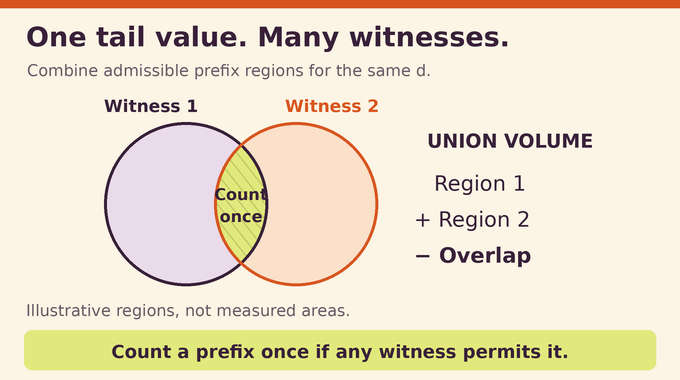
Let a tail witness be a particular choice of retained small primes and cofactor. Several witnesses may have the same totient . Each witness permits a region of continuous prefix coordinates.
Adding their volumes would count overlaps repeatedly. The correct object is the union of permitted regions, taken separately for each .
Suppose two tail witnesses permit the same prefix point. They generate the same output because their tail totients agree. If only one permits a different point, that point must still survive. Choosing one witness arbitrarily would therefore lose legitimate configurations.
Finite inclusion–exclusion implements this union exactly: add individual regions, subtract pairwise intersections, and continue through larger intersections. Intersecting witness regions means imposing the strongest threshold at each slack coordinate.
Uniqueness of the prefix and multiplicity of tails therefore coexist. The former removes large-scale collisions. The latter survives inside an exact local calculation. Counting the union preserves both facts without pretending that one representative tail describes every admissible prefix.
9. Constructing the Arithmetic Coefficient A(1;θ)
Reverse the tail indices by writing for . For a phase , put . The paper bounds the permitted tail primes and cofactors explicitly, leaving finitely many witnesses for each fixed , even across all phases.
Each witness contributes thresholds through for . Independent mean-one exponential variables encode the limiting slack constraints:
These are auxiliary probability variables, not an assumption that the original primes are independent. Like the distributions discussed in log-concave sampling, they provide a precise mathematical representation.
For constant weight one, sums the union probabilities over distinct tail totients, each weighted by , then multiplies by . The reciprocal weight comes from counting the largest prime. The prefactor comes from the ratio of prefix and full simplex volumes.
Write for the finite witness set for a fixed tail totient. Its union probability is given by:
Here counts witnesses in the subset. The maximum enforces every threshold in the intersection. Inclusion–exclusion turns each probability into exponential weights involving convergent series. Thus finite arithmetic data still involve an infinite analytic series. The approximants converge uniformly to as . Positivity and uniform bounds make the final approximation relative rather than merely additive. No evaluated decimal coefficient or practical convergence rate is supplied.
10. Why OpenAI’s Proof Establishes V(cx)/V(x) → c
One might substitute the asymptotic formula at two endpoints and cancel. That risks assuming regularity of the phase coefficient, which the theorem does not assert.
Instead, the paper counts the largest prime first. After fixing the remaining data, the allowed largest-prime range has an endpoint proportional to the output cutoff. The prime number theorem then produces a main term proportional to that cutoff.
For endpoints and , the proof uses the same parameters and representation mass. Their comparison establishes:
This is regular variation of totients with index one. It is proved before identifying the coefficient. Even when the integer changes between endpoints, no continuity assumption is smuggled into the comparison.
Unlike the algorithmic guarantee examined in counting perfect matchings, this limit supplies neither a selectable finite-input error nor a demonstrated runtime improvement. It describes asymptotic growth, without specifying where a desired numerical accuracy begins.
11. Least Preimages: Theorem 2.2 and the Questions Still Open
Define . For a fixed positive integer , let count totients whose least preimage satisfies . Notice the interval uses , not .
The weight measures an allowed interval fraction, evaluated at the tail ratio . It vanishes when and is positive when . Theorem 2.2 gives:
Here tends to zero. If some totient satisfies the seed condition , the coefficient is uniformly positive and has order , meaning comparable upper and lower bounds with constants depending on . Without such a seed, the count is identically zero. Positive cases are established for .
Whether is unbounded remains unresolved. A positive result for one seed does not supply seeds at every larger threshold. The weighted theorem identifies exactly what additional arithmetic evidence would be needed. The manuscript also supplies no empirical evidence for faster factoring, cryptographic attacks, or practical totient enumeration.
The published Lean scope covers the asymptotic equivalent, fixed scaling, and least-preimage results. Scope documentation is distinct from independently replaying the code, which this article has not done. Our Fermat formalization guide explains why matching a formal statement to the intended mathematics matters.
As checked on October 30, 2026, the Formal Conjectures tracker marks scaling solved while retaining the asymptotic-formula question as open. That classification does not erase the manuscript’s explicitly constructed equivalent, but it prevents declaring every interpretation of Problem 416 closed.
The number of totients now has a sharper mathematical description: continuous geometry for large primes, exact arithmetic for tails, and a union that counts outputs once. Follow Binary Verse AI for further source-led explanations of what AI mathematics proves and how its arguments work.
What are totient numbers?
Totient numbers are positive integers that occur as values of Euler’s totient function . For example, , so 8 is a totient. Not every positive integer occurs as a totient.
What is the difference between calculating a totient and counting distinct totient values?
Calculating gives one output for a particular integer. The totient counting function counts how many different outputs occur up to , even when several inputs produce the same output. The cutoff applies to outputs, not inputs.
How many distinct totient values are there below x?
Counting values up to and including , OpenAI’s Theorem 2.1 gives as . The scale and phase-dependent coefficient are explicitly defined through arithmetic constructions. This is an asymptotic equivalent, not an exact finite-cutoff count.
Why didn’t Ford’s earlier formula settle the number of totients?
Ford determined the correct order within bounded multiplicative uncertainty. That remaining uncertainty did not establish an asymptotic equivalent, where the ratio to a specified main term tends to one, or determine the precise fixed-dilation limit.
Does V(2x)/V(x) → 2 mean totient numbers become common?
No. Totient values have natural density zero: . The doubling result describes how their count changes between large multiplicative scales, not a positive density among all integers.
Is the coefficient A(1;θ) an ordinary constant?
It is a positive, bounded function of a phase parameter, constructed as the uniform limit of arithmetic approximations. The manuscript does not replace it with one fixed numerical constant or assert continuity of that function.
Did OpenAI’s proof resolve every open question about totients?
No. It establishes fixed scaling and an asymptotic equivalent, along with least-preimage results. Whether is unbounded remains unresolved in the paper. As checked on October 30, 2026, the Formal Conjectures tracker marks scaling solved but retains the asymptotic-formula part of Erdős Problem 416 as open.