

A machine may spend a trillion steps changing its tape, yet a simulator need not remember every changed cell to recover its answer. OpenAI’s September 25, 2026 preprint advances the time space tradeoff in Turing machines: a fixed deterministic machine with one writable tape can be simulated using two-fifths-power space, up to polylogarithmic factors, when a suitable time cap is supplied.
The result concerns memory, not speed. It recovers the control state and halting flag without constructing the final tape, and permits unrestricted simulation time. Its central idea combines shifted tape blocks, locally checked histories, and algebra that lets recursive computations borrow the same registers. The interesting question is how those pieces avoid quietly storing the entire computation elsewhere.
Table of Contents
1. What Is the Time Space Tradeoff in Turing Machines?
Let bound the source computation’s steps. Workspace counts the simulator’s writable memory in bits, excluding its read-only input. A one-tape Turing machine reads and writes its current cell, then moves its single writable head at most one position.
Direct simulation retains the visited tape. A space-conscious simulator can instead recompute information whenever needed. Think of answering whether a program accepted, rather than delivering its entire final memory dump. Those are different output obligations, just as finding a maximum matching differs from counting perfect matchings.
| Source | OpenAI preprint dated September 25, 2026. |
|---|---|
| Machine | One writable tape and head, plus a fixed number of read-only heads. All heads move at most one cell per step. |
| Memory | Work-space bits, excluding read-only input storage, bounded by two-fifths power of the cap times fixed logarithmic factors. |
| Output | Finite-control state and halting flag. The final writable tape need not be stored. |
| Time | Unrestricted. No useful simulation-time bound or practical speedup benchmark is supplied. |
2. The Square-Root Space Barrier and Previous Research
The classical one-tape bound is space, attributed to Hopcroft and Ullman in Williams’s account. Ryan Williams’s 2025 paper establishes space for deterministic multitape computations running in time .
These statements concern different source models. Williams also asked whether the one-tape exponent could fall below one-half by a fixed positive amount. Removing a logarithm would not answer that question. The new preprint lowers the power to two-fifths for its specified one-writable-head model, using ideas related to Cook–Mertz tree evaluation and Goldreich’s interpolation exposition.
3. What the OpenAI Proof Actually Establishes
Theorem 1 of the two-fifths-space manuscript gives:
Here is a fixed constant. The source machine is fixed and deterministic, with a finite alphabet, finite control, one writable tape and head, and finitely many additional read-only heads. All heads have fixed origins and unit movement. The binary cap satisfies .
One fixed accessor must supply every initial writable or read-only symbol within displacement using polylogarithmic workspace. The symbol contents are independent of the cap, and the condition covers speculative local computations too. Ordinary rescanning input access qualifies.
Halting states become absorbing. The returned outcome distinguishes halting by the cap from timeout. Constants may depend on the fixed machine and accessor. This is a precise Turing machine space complexity guarantee, not a claim that arbitrary input encodings are free. It measures a different resource from the input accesses counted in our quantum query complexity explainer.
4. Shifted Tape Blocks Reduce Boundary Crossings
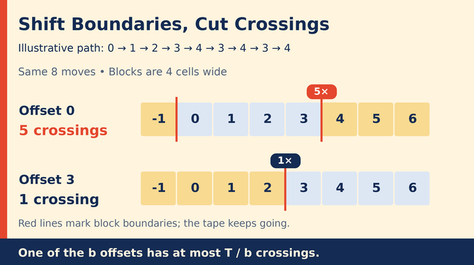
Partition the writable tape into blocks of width . There are offsets for placing the boundaries. Every moving step crosses a boundary for exactly one offset, while a stationary step crosses none. Summing crossing counts across offsets therefore gives at most .
By averaging, some offset has at most crossings. A visit runs inside one block until the head leaves, halts, or reaches the cap. That good partition needs at most visits.
For a worked example, take width four and head positions 0, 1, 2, 3, 4, 3, 4, 3, 4. Placing a boundary between cells 3 and 4 produces five crossings. Each other offset produces just one: the initial journey crosses its boundary once, then the oscillation stays inside a block. The four counts sum to eight, giving average two. A fortunate shift avoids repeated boundary traffic.
The simulator need not discover that offset cheaply. It tries them sequentially, reusing workspace, and discards offsets whose allotted visits do not reach halt or timeout. Every completed offset represents the same capped trajectory. Existence of one good offset guarantees eventual success.
The departure step writes the old block before moving. It reads the destination only on the next visit. This convention ensures each visit needs exactly one writable block, which becomes essential when consistency checks factor.
5. Local Replay Checks One Block at a Time
A short controller records the state, elapsed time, head displacements, and terminal flags. Its length is , since the number of heads is fixed.
Suppose a candidate transcript lists successive controllers. To check block A, load its starting contents and scan that list. Whenever the incoming controller selects A, simulate the visit, update A’s buffer, and compare the outgoing controller with the candidate. Other visits leave A untouched.
If the transcript claims A writes 1, then later revisits A expecting 0 without an intervening write, replay rejects it. The buffer preserves A’s changes across its visits even though other blocks are absent.
The underlying initial symbol accessor supplies a block when needed. Coordinates outside the reachable cap radius receive fixed filler symbols. Valid speculative controllers cannot move a head beyond that radius within their remaining time budget, so local replay never requires stronger input access than the theorem grants.
Repeat separately for every block. If all checks pass, induction forces every proposed controller to equal the deterministic reference computation. Each block’s returned buffer is then correct too. This avoids materializing the global tape tuple, much as our Existential Theory of the Reals explainer distinguishes defining a huge object from constructing it.
6. Controller Histories Become Factored Predicates
For a proposed continuation , each block supplies a Boolean predicate saying whether its replay agrees. Multiply those zero-or-one predicates: the product passes exactly when every block agrees.
Sum each candidate output multiplied by that product. At the true preceding history and true block contents, exactly one continuation passes. Consequently the sum returns the genuine next history.
The word “guess” describes an enumerated bit string. The simulator systematically evaluates candidates, rather than receiving advice from an oracle. There is no probabilistic failure allowance, unlike the randomized guarantee discussed in our subset sum analysis.
This separation between short shared history and independent block checks is special to one writable head. A visit that simultaneously reads two independently supplied writable blocks could test equality of their bits. The successful pairs 00 and 11 cannot be expressed as a product of separate one-block acceptance conditions.
The proof also defines the local Boolean operations on malformed strings. Algebraic lookup needs total functions, including values away from genuine histories. Invalid controller encodings receive prescribed behavior, and failed replay checks do not abort the bounded scan. Consistency is required at the semantic, genuinely defined inputs.
7. Epochs and Rounds Limit Retained Guesses
Choose three coordinated scales:
An epoch contains visits, divided into rounds of visits. It takes epochs to cover the allotted visits. Dummy stationary visits pad the computation only after halt or timeout.
An epoch history stores its incoming controller and the outgoing controllers accumulated so far. A block checkpoint describes that block at the epoch’s start. Either fits a common padded word of width .
A round proposes controllers, costing guess bits. Its checks replay the entire current epoch prefix from each starting checkpoint, so earlier writes remain accounted for. Replaying only the new suffix from the old checkpoint would be wrong.
| Tape Block | cells, retained as one local buffer during replay. |
|---|---|
| Epoch History | At most controller records, packed into a word of bits. |
| Round Candidate | controller records, costing bits when retained. |
| Epoch Count | epochs for the chosen visit budget. |
| Checkpoints | Defined for every epoch and block, but regenerated through dependencies rather than stored as a complete array. |
For example, if , an epoch has nine visits and three rounds. After round two, its history contains the incoming controller plus six outgoing controllers. The next candidate supplies only three new controllers, yet each block check scans the full nine-visit proposed prefix. This illustrates the organization, not a performance measurement.
The histories and checkpoints define a dependency graph. They are mathematical word values, not an array kept in memory. Their identifiers and dependencies can be generated using short counters.
8. Polynomial Interpolation Cancels Register Baselines
The algebra uses finite fields of characteristic two, where adding a value twice cancels it. Field elements need only bits, with the field chosen large enough for the interpolation degrees.
First augment every -bit word with a final coordinate equal to one. A Boolean lookup becomes a polynomial homogeneous of degree in each augmented argument. A basis factor uses for a required one and for a required zero. Multiplying these factors identifies a particular Boolean word.
Homogeneity means every monomial has the same total degree. For a homogeneous polynomial of degree , suitable Lagrange weights satisfy:
Here contains distinct field elements. The weights extract the coefficient of degree in the sampling variable. That coefficient depends on the desired vector , not the arbitrary register baseline .
For a tiny example, take over a characteristic-two field with at least four elements. Then . Interpolating from three distinct samples extracts and eliminates . The full proof applies the same principle to multicoordinate lookup polynomials.
For the weights, take the reciprocal of the product of all differences from the other sample points. Distinctness makes those denominators nonzero. This coefficient-extraction argument uses neither derivatives nor factorials, so characteristic two causes no division-by-factorial problem.
In a round update, the history argument appears in the candidate-output polynomial and all predicates, giving homogeneous degree . Here counts represented blocks. The evaluator extracts each block factor at a fixed shifted history, multiplying it into a scalar accumulator. Outer interpolation then removes the history baseline. It never needs to retain a list of all factor values.
Unlike unrestricted complex arithmetic in our Fourier transform complexity explainer, these field operations have explicit bit-space costs. Even constant-one lookup functions retain homogeneous extensions: the augmentation coordinate cannot simply be discarded.
9. Shared Registers and Weighted Dependency Paths
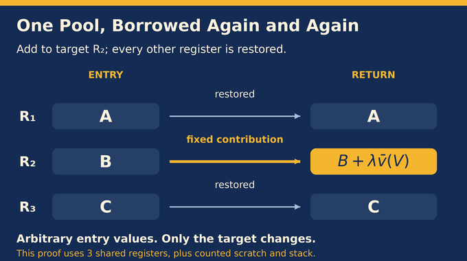
Lemma 5 supplies the evaluator. Its procedure adds a scaled, fixed semantic word value to target register :
Here identifies a word, is a field scalar, and the bar denotes the augmented value. Every other register returns to its entry value. Crucially, the contract holds for arbitrary contents throughout the register pool. A child can borrow the caller’s inputs or partially accumulated output and restore them before returning. This application needs three shared vector registers, rather than fresh vectors at every recursion level.
Interpolation shifts registers by semantic child values, evaluates local lookups, and reverses the shifts. Lookup scratch is released before recursion. Only necessary scalars, indices, and active guesses survive on the ordinary stack.
The arbitrary-baseline condition is what makes borrowing safe. A child sees whatever vectors its ancestors currently hold, rather than a specially cleared workspace. Its translation depends on the fixed semantic word, independently of those mutable vectors. Applying the reverse translation restores its target even if other registers were borrowed between the forward and reverse calls.
The scheduling distinction does the heavy lifting. Calls to the preceding history occur outside the candidate loop, so they retain no large guess. Calls to epoch-start blocks retain the current -bit candidate. Each such block depends only on earlier epochs, preventing another expensive guess edge in the same epoch along that path.
Lemma 5 charges edges accordingly: ordinary and preceding-history edges have weight one, while block dependencies cost . Maximum weighted path length, plus word width, bounds space up to logarithms. Across an epoch a path pays for at most history steps and one large guess. Repeated sequential calls increase time, not simultaneously occupied memory.
10. Why the Exponent Is Two-Fifths
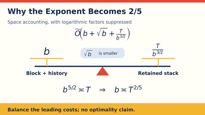
Combining the word width and weighted stack gives:
The tilde suppresses fixed logarithmic powers. Expanding exposes the competing terms:
Larger blocks increase the buffer and history cost but reduce the epoch-related stack cost. Balance the dominating terms:
The square-root term is smaller at this choice. This produces two-fifths-power space, with logarithms restored, rather than a log-free endpoint.
The paper also varies block width , epoch length , and round length independently. Ignoring logarithms, word storage is and the stack estimate is . Choosing near balances those stack contributions. Keeping both and within storage budget leaves that estimate at least .
Thus retuning these three scales within the displayed accounting does not establish a better power. It is no optimality theorem for other simulators. As in our quadratic sensitivity analysis, the precise direction of a bound matters. This paper provides an upper bound, unlike the exclusions examined in our quantum circuit lower bounds explainer.
11. Consequences, Limits, and Lean Verification
An unknown halting time is handled by caps 2, 4, 8, and onward, discarding workspace between trials. If the source halts at time , the first sufficient cap is within a constant factor of . This requires the symbol-access condition for every cap and identical underlying initial contents across trials.
The paper derives space-hierarchy consequences. For space-constructible , some deterministic -space languages escape every fixed one-writable-tape time bound , where . These are class noncontainment statements in the specified model, not per-input-length lower bounds.
The multitape comparison separately achieves square-root-type space. A standard quadratic-time one-tape conversion would instead yield a four-fifths exponent in the original time parameter. Neither route gives two-fifths space for arbitrary RAM programs.
OpenAI’s published Lean scope covers the capped and unknown-time main statements. It explicitly excludes general multitape simulation, hierarchy consequences, and bounded-space halting. Readers can compare our explanation of Lean proof checking for why matching the formal statement matters. This article does not report an independent Lean build.
No useful simulation-time bound or practical benchmark is supplied. Developers should read this as a new memory upper bound, not an optimization recipe. Our 3SUM analysis examines the separate question of reducing a running-time exponent. The time space tradeoff in Turing machines becomes more surprising because consistency, interpolation, and storage lifetimes work together. Follow Binary Verse AI for research explanations that unpack those mechanisms alongside their assumptions.
What is the time–space tradeoff in a Turing machine?
It describes how additional computation can reduce the memory needed to obtain an outcome. The OpenAI proof establishes an asymptotic space bound for simulating a fixed deterministic machine with one writable tape and head, under the paper’s symbol-access assumptions.
Why is better than ?
The exponent falls from 0.5 to 0.4, giving an asymptotically smaller power of . The theorem also includes fixed polylogarithmic factors, so the exponent alone does not establish practical savings for every finite input.
How can a deterministic simulator use guessed computation histories?
It evaluates candidate histories through exact consistency checks. At the true preceding history and block contents, only the actual next controller continuation passes all checks. Candidates are evaluated deterministically, without a nondeterministic oracle.
Does the OpenAI proof make Turing machine computations faster?
No. The theorem improves workspace usage, not execution speed. Simulation time is unrestricted, and the paper supplies no useful simulation-time bound or practical speedup benchmark.
Does the simulator need to know when the original machine halts?
Not necessarily. If the original computation eventually halts and the symbol-access condition holds for every cap, the simulator tries successively doubled caps while reusing memory. The initial symbol contents must remain independent of the cap.
Does the two-fifths-space result apply to multitape machines and RAM computers?
Not directly. The main theorem requires one writable tape and head. The paper separately gives a square-root-type multitape simulation. Standard quadratic-time conversion to one writable tape yields a four-fifths-space exponent in the original time parameter, not two-fifths. Arbitrary RAM consequences are not established by Theorem 1.
Has the OpenAI proof been verified in Lean?
OpenAI’s published Lean documentation covers the time-capped main theorem and the version for unknown halting time. General multitape simulation, space-hierarchy consequences, and bounded-space-halting results are outside those selected formalized statements. This article does not report an independent Lean build.