
Counting an elliptic curve’s points modulo primes produces an arithmetic fingerprint. Modularity says that an entirely different object, an automorphic representation, reproduces that fingerprint and its deeper local structure. OpenAI’s October 4, 2026 manuscript claims elliptic curve modularity for every elliptic curve over every imaginary quadratic field, removing restrictions that earlier results still required.
The proposed bridge is geometric prime switching: construct related Galois representations inside one family of curves, then transfer automorphy through three carefully controlled congruences. This is a preprint claim, not a report of independently certified correctness. Its interest lies in how geometry makes existing lifting theorems reach the remaining cases.
Table of Contents
1. Elliptic Curve Modularity: What the OpenAI Proof Establishes
Theorem 1.1 of the modularity manuscript assigns each curve a weight-zero isobaric automorphic representation of , with trivial central character. Here packages all completions of the number field. “Isobaric” allows the decomposable representations needed in some complex-multiplication cases.
The right side is the curve’s two-dimensional étale cohomology, carrying its arithmetic symmetries. The left side is the Galois representation associated with the automorphic object, using a coefficient identification . The assertion holds for every coefficient prime , with matching local parameters, rather than merely matching selected point counts.
Think of modularity as an exact translation between arithmetic and harmonic analysis. A successful translation must preserve how the object behaves at every completion of the field. Agreement at many convenient primes is compelling evidence, but the theorem promises a complete dictionary, including the difficult local entries.
| Question | Precise Answer |
|---|---|
| Which curves? | Every elliptic curve over every imaginary quadratic field. |
| What compatibility? | All finite local factors, including bad reduction, and the prescribed complex-place parameter. |
| Which automorphic type? | Cuspidal for non-CM curves; induction or an isobaric sum in the CM case. |
| What new mechanism? | One integral geometric construction supporting three automorphy lifts. |
| What evidence? | An OpenAI preprint. Full independent verification is not established by the sources examined. |
OpenAI’s release announcement attributes the collection to an internal frontier model. That attribution describes provenance, not mathematical acceptance, a distinction familiar from our coverage of AI mathematical proofs.
2. The Original Problem: Why Imaginary Quadratic Fields Were Different
An imaginary quadratic field has the form , with a positive squarefree integer. For example, adjoining gives the Gaussian rationals. “Imaginary” describes the field’s embeddings, not a speculative kind of arithmetic.
An elliptic curve is a smooth genus-one curve with a chosen origin. Its torsion points carry actions of , the absolute Galois group recording algebraic symmetries over . Passing to cohomology organizes these actions into two-dimensional representations, one for each coefficient prime.
Over the rationals, modularity is classically expressed through weight-two modular forms. Over imaginary quadratic fields, Bianchi forms and automorphic representations of supply the corresponding language. Their arithmetic quotients involve hyperbolic three-space, and relevant cohomology occurs in multiple degrees. The classical argument therefore does not transfer unchanged.
At a good place with residue field of size , the basic arithmetic datum is . The symbol counts points, including the origin. A matching Hecke polynomial has coefficients determined by this trace and . Bad reduction requires additional information because this simple good-place description no longer captures the whole local representation.
For example, over has eight points including the origin, giving trace . Modularity predicts the matching automorphic datum.
3. The Previous Barrier: Why Modularity Was Still Incomplete
Wiles and Taylor–Wiles established modularity for semistable elliptic curves over the rationals. Breuil, Conrad, Diamond, and Taylor completed the rational theorem. This history underpins the mathematics behind Fermat’s Last Theorem.
For imaginary quadratic fields, Caraiani and Newton’s theorem already covered every curve over infinitely many fields, including those with . More precisely, their field criterion required the modular curve to retain rank zero over the field. Their broader CM-field results also supplied modularity under suitable mod-3 or mod-5 image hypotheses.
Residual means reducing a representation to finite characteristic. If that reduction is reducible, it preserves a line, and a lifting theorem requiring irreducibility cannot simply be invoked. Small-characteristic image restrictions left awkward cases outside the available route.
Potential modularity was also known much more generally. It permits enlarging the ground field. Actual modularity must return to the specified field, an essential extra demand. The new manuscript builds on these achievements, especially Caraiani–Newton, rather than replacing their machinery.
4. The New Argument: Geometric Prime Switching
Begin with a non-CM curve written , where is a separable cubic. Serre’s open-image theorem permits a prime whose torsion image contains . Set and , adjoining the th roots of unity.
The working field is CM, meaning a totally imaginary quadratic extension of a totally real field, and it does not contain a primitive fifth root of unity. That last detail enables the initial modularity theorem later.
This quadratic twist acquires the marked point . Twisting preserves the underlying curve after a quadratic extension while changing its arithmetic action by a character. Our Goldfeld conjecture explainer develops this family relationship in a different setting.
The plan is to connect the twist to an auxiliary elliptic curve already accessible to modularity theorems. Intermediate representations need not themselves come from elliptic curves. They must retain the precise properties those theorems require.
This is why the larger geometric object is useful. Its Jacobian, an abelian variety encoding degree-zero divisor classes on the curve, holds many two-dimensional pieces under one roof. The construction can compare those pieces integrally while arranging their local behavior together. Choosing unrelated auxiliary representations would leave both kinds of compatibility to be proved from scratch.
5. Constructing Cyclic Covers and Rank-Two Galois Systems
Put , meaning multiplication by in the elliptic-curve group. Choose a rational function with divisor , normalized by at the origin. The weighted group sum vanishes, which makes this divisor principal.
Here is a point on . Away from excluded parameters, the normalized cover branches only at and . The other divisor orders are multiples of , so they cause no ramification. Riemann–Hurwitz gives , hence genus .
Rotations multiply by roots of unity. The involution reverses those rotations, giving dihedral symmetry. For a rotation character , take its eigenspace:
Each piece has dimension two. Pairing opposite characters and using the involution gives determinant , where the cyclotomic character has Hodge–Tate weight minus one in the paper’s convention. Each piece has weights zero and one. The trivial character recovers . An order-three character recovers , with the Jacobian of the genus-one quotient .
6. Two Degenerations: How Geometry Supplies the Missing Conditions
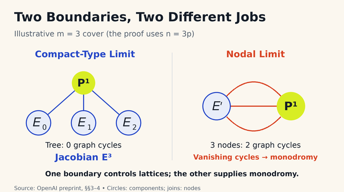
After pulling the parameter back to the original elliptic curve, move its marked point toward the origin. The limiting cover has a rational central component attached to copies of . Its graph is a tree. Consequently its Jacobian has compact-type limit , a product with no toric contribution.
A second collision joins one elliptic component and one rational component at nodes. Loops around these singular fibers act on homology through vanishing cycles, the loops that shrink at a node. Monodromy records how cycles change as the parameter travels around a singular value. A unipotent transformation has identity eigenvalues but can still shear vectors.
| Boundary | Geometry | Proof Contribution |
|---|---|---|
| Marked point approaches the origin | A rational component with elliptic leaves; graph has no cycles. | Product Jacobian and integral control near that fiber. |
| Opposite branch points collide | Two components joined at nodes; graph has independent cycles. | Explicit vanishing cycles and nontrivial monodromy operators. |
A slit construction identifies an integral basis on the sheets. It proves freeness over the group ring, not merely over rational coefficients:
In this same basis, horizontal and vertical degenerations yield opposite unipotent transformations. On a nontrivial character their off-diagonal coefficient is, up to sign, , where is the rotation eigenvalue. Working in one basis matters: triangular matrices described in unrelated bases would not establish the required irreducibility.
7. The Crucial Congruence Chain: Why Switching Primes Works
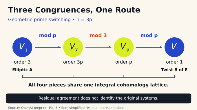
Choose characters of order three and of order , and write . A root of unity of prime-power order reduces to one in that prime’s characteristic. This gives three links:
Thus the order- character disappears in the first link, the order-three character disappears in the second, and the remaining order- character disappears in the third. Each congruence identifies semisimplified residual Galois representations, not the original characteristic-zero systems.
The integral lattice makes that statement legitimate. Ordinary eigenspace projectors divide by , precisely the wrong operation when reducing at three or . Instead, evaluate the free integral group-ring module at each character before reducing. Characters with identical residual values then produce identical residual modules. Rational information alone would lose this control, a related concern in our discussion of the exact BSD formula.
8. Controlling Local Reduction, Irreducibility, and Genericity
The parameter must satisfy every lifting condition simultaneously. Near the compact-type fiber, sufficiently deep finite torsion stays locally constant. After securing semistability, the possible full Frobenius polynomials form a finite set. Deep enough torsion comparison therefore preserves toric rank and, in good reduction, Newton slopes.
At places above , the Jacobian is arranged to follow the original curve’s potential reduction type. Ordinary good reduction makes every character piece potentially crystalline and ordinary. Supersingular good reduction gives slopes one-half and excludes potential ordinarity. Potentially multiplicative reduction produces a totally toric Jacobian, forcing rank-one monodromy on every two-dimensional piece.
Meanwhile the opposite unipotents have different invariant lines, giving absolute irreducibility. Decomposed genericity asks for an unramified rational prime splitting completely in , where neither Frobenius eigenvalue ratio equals the prime’s residue in the coefficient field, at every place above it. The construction uses primes congruent to one in the residual characteristic, reducing this to distinct eigenvalues.
The inequality also has a concrete geometric role. In characteristic three, failure of a selected monodromy product to have distinct eigenvalues would force a primitive th root to satisfy a polynomial of degree at most four. Its order would then divide for some , at most eighty, contradicting the chosen prime.
Chebotarev supplies suitable primes, a splitting principle also encountered in our primitive-root research coverage. Hilbert irreducibility with weak approximation preserves the needed finite monodromy images while meeting local open conditions. Restriction of scalars handles both conjugate parameter families together, preventing a check at one place from overlooking its conjugate.
9. The Three Modularity Lifts: From the Auxiliary Curve to E
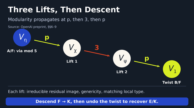
The specialized auxiliary curve is non-CM. Its mod-5 representation has the required irreducibility and decomposed genericity. Since does not contain a primitive fifth root of unity, the elliptic starting theorem supplies automorphy of . Five starts the process. It is not a fourth switching step.
| Known Input | Prime and Target | Residual Justification |
|---|---|---|
| : lift to | Order-three cover in characteristic . | |
| 3: lift to | Order- cover in characteristic 3. | |
| : lift to | Large mod- image of the original curve and its twist. |
At every transition, determinants, Hodge–Tate weights, finite ramification, and potential semistability are already supplied by geometry. The residual representations are absolutely irreducible over the required cyclotomic extension and decomposed generic. The lifting prime is three or , never five.
Local conditions must match too. In potentially good cases, both sides have matching ordinarity behavior and the input automorphic parameter has zero monodromy. In toric cases, neither side is potentially crystalline, and the input is an ordinary quadratic or trivial twist of Steinberg. Compatible Frobenius polynomials, Chebotarev, and semisimplicity identify the system across coefficient primes, allowing each output to become the next input.
For researchers checking the argument, the local comparison deserves particular attention. For intermediate systems, the proof first uses compatibility of the underlying semisimplified Weil representations. It then invokes purity or genericity to determine the automorphic monodromy. Assuming full monodromy compatibility at that stage would skip a necessary justification.
10. Descending Back to the Original Imaginary Quadratic Field
After the lifts, only is known to be modular. Stopping here would establish the result over the wrong field. Because is abelian, it can be traversed downward through cyclic extensions of prime degree, with CM fields at every stage.
At one step, the Galois representation already extends downstairs. Strong multiplicity one makes its upstairs automorphic representation invariant, so cyclic base change gives a descent. But the descended representation can differ from the desired one by a finite-order character.
Absolute irreducibility and Schur’s lemma identify precisely that scalar discrepancy. Twisting by the inverse Hecke character removes it. Repeating the correction down the tower proves modularity of . Applying the original quadratic twisting character then recovers . Descent is an argument with its own hypotheses, not a change of address.
11. The Final Theorem: Local L-Factors, CM Curves, and What Follows
With unitary automorphic normalization, the manuscript concludes:
These L-functions assemble local arithmetic factors into global analytic objects. The half-unit shift records a convention. At a good finite place, compatibility recovers the reduced curve’s point count. At bad places, the Frobenius-semisimplified Weil–Deligne comparison also retains inertia and monodromy. At the complex place, the parameter has Hodge types and .
CM curves follow a separate classical route through Hecke characters. When the CM field is not contained in , automorphic induction applies. When it equals , the representation is an isobaric sum. CM means extra endomorphisms, a structure discussed in our CM abelian-variety explainer, not the absence of difficult mathematics.
As checked on October 21, 2026, the public formalization catalogue did not identify a full Lean formalization of this manuscript. The supplied paper provides no performance benchmark or practical cryptographic algorithm. Its theorem does not establish unrestricted BSD or modularity over all number fields.
The useful contribution to examine is a reusable architecture: one integral family connects awkward representations to accessible ones while preserving every lifting hypothesis. Follow Binary Verse AI for source-led analysis of elliptic curve modularity, proof verification, and the mathematics behind AI research headlines.
What is a modular elliptic curve?
An elliptic curve is modular when its arithmetic Galois representations correspond to suitable automorphic representations. Over , this is classically described using modular forms. Over imaginary quadratic fields, the relevant objects are automorphic representations of over the number field.
What is the modularity theorem, and how does OpenAI’s proof extend it?
The classical theorem establishes modularity for every elliptic curve over . OpenAI’s October 4, 2026 preprint claims the corresponding result for every elliptic curve over every imaginary quadratic field, including local compatibility. That manuscript claim should be distinguished from independently verified acceptance of the full argument.
Why had elliptic curve modularity over imaginary quadratic fields remained unresolved?
Earlier results established modularity in many cases but required residual-image hypotheses or restrictions on the base field. Certain reducible mod-3 and mod-5 representations blocked a direct application of the available lifting route. Potential modularity after extending the field did not by itself establish modularity over the original field.
What is geometric prime switching in the OpenAI proof?
It constructs cyclic covers whose cohomology yields related two-dimensional Galois systems. Their reductions agree at selected primes. After verifying residual-image and local-reduction hypotheses, automorphy transfers through these systems from an auxiliary elliptic curve to a twist of the original curve.
Why does the proof use primes 3, 5, and ?
Five establishes modularity of the auxiliary elliptic curve. A sufficiently large prime supplies favorable residual-image properties. Three and then govern the three congruences and automorphy lifts, in the order . Their roles are distinct.
What does mean in the proof?
It means the Galois representations have isomorphic semisimplified reductions in characteristic , using compatible coefficient embeddings. The congruence comes from evaluating the same free integral cohomology module at characters whose reductions coincide. It does not identify the characteristic-zero representations.
Does the OpenAI proof cover CM elliptic curves and bad reduction?
Yes, those cases are included in the manuscript’s theorem. CM curves are handled separately using Hecke characters, automorphic induction, or an isobaric sum. At bad-reduction places the statement compares the relevant Frobenius-semisimplified Weil–Deligne parameters, including inertia and monodromy, rather than only good-prime point counts.