
A square of quantum spins can contain a vast number of possible states. The striking question is how much of that complexity a ground state actually uses to connect the square with its surroundings. OpenAI’s September 24, 2026 manuscript presents a proof of the 2D area law: under fixed locality bounds, a unique ground state and a size-independent global spectral gap, entanglement entropy grows at most with the region’s boundary, not its interior.
Released in OpenAI’s October mathematics collection, the 90-page argument targets a long-standing gap-to-entanglement conjecture. Its distinctive achievement is dispensing with spectral-gap assumptions for smaller subsystems. This is a preprint claim requiring scrutiny, not a quantum-simulation benchmark.
1. 2D Area Law: The Original Entanglement Problem
A Hamiltonian specifies a quantum system’s energy and interactions. Its ground state is a lowest-energy state. Locality limits which sites can interact directly, while a spectral gap separates the ground energy from excited energies. Neither description immediately limits the information shared across a spatial cut.
The 2D area law conjecture asks whether those ingredients force boundary-sized entanglement. The manuscript’s answer is affirmative for its stated finite-dimensional square-lattice class, including frustrated interactions and irregular regions. Its Theorem 1.1 and full proof provide the precise target.
Table of Contents
1.1. 2D Area Law Research: Key Facts
| Question | Manuscript Scope |
|---|---|
| What is bounded? | Von Neumann entropy of every site subset. |
| Which geometry? | Any finite induced square-lattice domain. |
| What spectral input? | Unique ground state and a positive full-system gap. |
| What stays fixed? | Local dimension, interaction range, strength and gap lower bound. |
| What is established publicly? | A released preprint. Family 265 has no linked Lean formalization in the checked catalogue. |
2. Area vs Volume Scaling: What the Entanglement Entropy Bound Means
Let be a set of sites and the normalized pure ground state. Tracing out the remaining sites gives the reduced density matrix . Its eigenvalues describe the weights in the entanglement spectrum. Von Neumann entropy averages their negative logarithms:
The paper uses natural logarithms, so entropy is measured in nats. Its entanglement entropy area law reads:
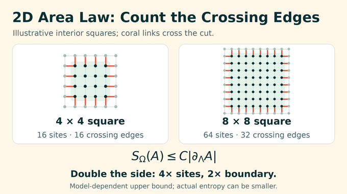
Here counts nearest-neighbor edges crossing from the region to its complement within the physical domain. depends on the fixed model parameters. For an interior square with side , there are sites but crossing edges. Doubling the side quadruples the volume and only doubles the boundary.
This is an upper bound, not a claim that every state saturates it. A product state has zero entanglement. Also, ‘two-dimensional’ describes spatial geometry, not a two-dimensional Hilbert space. Qubits are allowed, but so are other fixed local dimensions.
3. The Previous Barrier: Hastings’ 1D Proof and Earlier 2D Bounds
Hastings’ 2007 one-dimensional theorem established a length-independent entropy bound for gapped local chains. In two dimensions, a cut grows with the lattice, making the balance between suppressing excitations and controlling entanglement much harder.
Anshu, Arad and Gosset’s earlier subvolume result bounded rectangular-region entropy by , with the boundary size. It assumed a unique frustration-free ground state, plaquette-projector interactions and a uniform local gap. Subvolume is progress, but a boundary exponent of five-thirds still exceeds one.
Their subsequent vertical-cut theorem, despite its ‘area law’ title, gives the near-linear bound , where is cut length. OpenAI’s manuscript distinguishes that estimate from a strict constant-times-boundary law. The older result also retains frustration-free and local-gap assumptions.
A gap implies decay of connected correlations between separated observables under standard locality hypotheses. Entropy, however, depends on the entire reduced spectrum. Small ordinary correlations are not a shortcut to the required entropy inequality.
4. OpenAI’s 2D Area Law Theorem: Exact Statement and Assumptions
Take a finite site set in the integer square lattice, retaining every nearest-neighbor edge between included sites. At each site place a Hilbert space of dimension . Interactions have the form:
Every term is Hermitian and acts only on its support . The fixed integer bounds that support’s diameter in induced-graph distance, and bounds its operator norm. The manuscript indexes one term per support, allowing zero terms. Fixed range and square-lattice degree then bound the total interaction strength around each site.
Assume a unique normalized ground vector, up to phase, with ground energy and gap lower bound . The conclusion holds for every region with the same finite , independent of the domain’s size and shape.
Those dependencies matter. The theorem does not promise a universal numerical entropy coefficient. Increasing local dimension or allowing the gap to shrink with system size leaves the fixed-parameter guarantee. It also assumes the gap rather than supplying a procedure to certify it.
An empty crossing boundary is a useful consistency check. If a region is a union of disconnected components, induced-graph finite-range terms cannot connect it to the other components. Uniqueness forces the full ground state to factor across that separation, so the entropy is zero. The theorem’s boundary convention captures this case without an extra correction.
5. Global Spectral Gap vs Local Gap: Why This Distinction Changes Everything
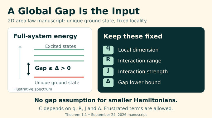
The full-system spectral assumption is an operator inequality:
is the identity. Every vector orthogonal to the ground state therefore costs at least in energy above . For a family of larger systems, the same positive lower bound must apply throughout.
A local-gap assumption additionally controls Hamiltonians built from selected subsets of interaction terms. Cutting out a region can change its spectrum and create low-energy boundary behavior. A gap for the original system does not automatically provide these extra guarantees.
Frustration-free means one ground state minimizes every interaction separately. Frustrated systems require compromises between terms. The OpenAI 2D area law proof permits those compromises, so its spectral gap area law connection applies under substantially weaker hypotheses than the earlier restricted 2D results.
Our Haldane gap explainer examines the complementary difficulty: proving a size-independent gap for a particular quantum model. Here that property is the input.
6. Proof Stage 1: Marginal Spectral Tails and the First Subvolume Bound
Choose a positive marginal eigenvalue . Its surprisal is , and entropy is the average surprisal. The first analytic step bounds fluctuations of this quantity using the global gap. Controlling spectral tails means rare eigenvalues cannot contribute unchecked amounts of entropy.
The proof tilts the ground vector by applying an inverse power of a marginal density operator on its positive spectrum. This reweights Schmidt components. Comparing the tilted vector’s energy cost with its norm turns the spectral gap into a concentration estimate. Zero eigenvalues are treated separately rather than silently inverted.
Next, nested rectangles and intervening buffers yield a conditional-entropy discount. A buffer reduces the entropy cost attributed to adding another region. Optimization of positive-operator products gives an initial ‘safe-box’ estimate:
is an ambient box of side at most , sufficiently separated from the original cut. Because is below one, the exponent is below the two-dimensional volume exponent. This first bound is deliberately weaker than the final area law. It supplies the entropy control needed to improve itself.
7. Proof Stage 2: Positive Constraints and Local Spectral Filtering
The original interaction terms need not annihilate the ground state individually. The proof constructs replacements that do. Smooth spectral filtering removes ground-to-excited matrix elements, and subtracting each term’s ground-state expectation centers the resulting Hermitian operator.
The centered filtered terms sum to the original Hamiltonian minus its ground energy. Taking their absolute values produces positive constraints. This is the crucial gap-preserving step: a Hermitian operator’s absolute value dominates the operator itself, so the new positive sum dominates the shifted Hamiltonian after normalization.
Each constraint annihilates the ground vector, and their sum retains a size-independent global gap. They are quasi-local, meaning they have spatial tails rather than exact finite support. Propagation bounds and smooth filtering control those tails. Truncation near a finite set has an error independent of the total system volume.
The distinction between exact annihilation and approximate spatial localization is essential. Treating the constraints as strictly local projectors would discard the errors that later stages must track. The construction creates useful operators without assuming the original model was frustration-free.
8. Proof Stage 3: Symmetric Replicas, Schur–Weyl Duality and Entropy Metrics
The proof now introduces many copies of the system. Symmetric replicas are vectors unchanged by permuting those copies. Schur–Weyl duality organizes tensor powers into representation sectors whose labels encode information about marginal eigenvalue distributions.
This translates spectral information into operator estimates. Positive operator metrics assign weights to different partitions, while interpolation compares those weights when a small subsystem moves between parts. Weighted operator geometric means organize sequences of such changes.
The important purpose is joint accounting. The transported states measure both information gained and excitation energy spent. Without that shared family of states, an entropy estimate and an energy estimate might concern incompatible objects and prove nothing together.
As replica number grows, logarithmic norms per copy can be compared with marginal entropies. Finite quantum de Finetti measures and symmetrized-observable estimates support the return to one-copy quantities. These replicas are proof devices, not a proposal to manufacture many quantum samples.
Entropy also drives our Courtade–Kumar analysis, although its Boolean-noise problem is different. Here the bridge must connect quantum information to physical excitation energy.
9. Proof Stage 4: Auxiliary-Pair Norm Comparisons and Scanning Collars
An auxiliary entangled pair anchors two estimates of a filtered vector’s norm. Its dimensions are selected from a high-probability portion of the target’s Schmidt spectrum. An entangled-pair projection gives one comparison. The other uses the gap: sufficiently low physical energy forces most copies close to the ground state.
The scanner moves partitions through a collar, a surrounding buffer zone. A randomized schedule makes any particular interaction rarely straddle a moving boundary. This supplies an interpolation with controlled energy, allowing the norm comparisons to constrain information shared across the collar.
Repeated improvement first lowers the safe-box entropy exponent. Sharper comparisons then bound mutual information between a target and the region beyond a sufficiently wide collar. For disjoint systems, mutual information is:
It measures total dependence, including classical and quantum correlations. The intermediate collar bound is sublinear in the target scale, not yet arbitrarily small. Nor does it apply to every imaginable shape without qualification: the estimates use specified unions of rectangles and triangles. The final geometry must fit these templates.
10. Proof Stage 5: Amplification Through Localized Operators and Unitary Decoupling
The next task is to make the collar error small enough to sum over many regions. Typical spectral subspaces first produce a candidate operator that restores a target transferred to an auxiliary reference. The previous mutual-information bound controls that operator’s norm.
Products of positive contractions derived from the constraints preserve the ground state while suppressing excited components. Their localization is proved alongside their decay. Polar decomposition then supplies a unitary acting near the target, with the reference and distant physical system untouched.
Comparison with a state where reference and remote system are independent converts this construction into a sharper mutual-information estimate. For any fixed desired inverse-polynomial accuracy, a sufficiently large scale and an enlarged, still sublinear collar achieve it.
This is an asymptotic estimate with constants and thresholds depending on the requested error power. It is not a measured decay curve or a recipe with reported runtime. Nevertheless, the strengthening is decisive: the region construction can now accumulate information errors without paying a volume-sized penalty.
11. Completing the Proof: Two Region Families and Entropy Cancellation
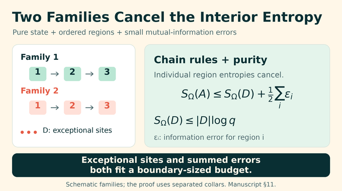
The final step partitions the region into two ordered families of separated pieces, plus exceptional sites. Each piece’s collar avoids the complement and all earlier pieces in its own family. Sparse strips and recursive repairs around point contacts enforce that separation even for awkward boundaries.
Let denote the exceptional sites and each piece’s mutual-information error. The manuscript’s entropy-cancellation lemma gives:
Two applications of the entropy chain rule, together with purity and subadditivity, cancel the individual piece entropies. What remains is the exceptional-set entropy and the summed errors. Each exceptional site contributes at most , and the number of such sites is proportional to the original boundary.
The geometric construction also makes the amplified errors summable within the same boundary budget. This closes the argument for arbitrary site subsets. Holes and disconnected domains are handled through induced-graph locality rather than by pretending paths can cross missing sites.
The proof succeeds because geometry and information estimates cooperate. Decaying correlations alone never perform this cancellation.
12. What OpenAI’s 2D Area Law Establishes and What It Does Not
The result covers arbitrary regions in finite induced square-lattice domains, including holes and disconnected pieces. It does not establish the analogous theorem in three dimensions, for gapless systems, or for arbitrary choices within degenerate ground spaces.
For a numerical developer, the practical question remains model-specific: do the chosen interactions satisfy the bounds, is the gap certified, and can a useful tensor representation actually be found? The paper answers the structural entropy question. It reports no simulation timings, hardware advantage or training-speed improvement, so those claims would need separate evidence.
12.1. Entropy Bounds, Representation and Computation
| Result | What It Provides | What It Does Not Establish |
|---|---|---|
| Area-law manuscript | Boundary-sized entropy under Theorem 1.1’s assumptions. | An efficient ground-state simulation algorithm. |
| PEPS companion | Polynomial bond dimension on open square grids, with global vector error at most the inverse side length. | Efficient tensor construction or contraction. |
| Public verification record | A manuscript available for checking; no family-265 Lean link in the checked catalogue. | Independent referee acceptance or a complete machine-checked proof of this theorem. |
The polynomial-PEPS companion theorem assumes on-site and nearest-neighbor interactions on an open grid. It uses additional collar estimates and compression arguments, not the entropy inequality alone. Small representation size does not establish cheap construction or contraction.
As checked on October 13, 2026, OpenAI’s repository warns that unformalized results may contain issues. Its catalogue links no Lean formalization for this family, and the checked revision history lists no area-law correction. That supports cautious status reporting, not a declaration of independent verification. The release announcement attributes the collection to an internal frontier model.
Our guides to AI mathematical proofs and formalization scope explain why checking the exact theorem matters. For researchers, the useful advance is the proposed gap-to-information machinery. Follow Binary Verse AI for source-led updates on the 2D area law, its verification and its computational consequences.
What is the 2D area law for entanglement entropy?
The 2D area law bounds a region’s ground-state entanglement entropy by a constant times its lattice boundary size, rather than its number of sites. OpenAI’s manuscript states this theorem for unique gapped ground states of bounded, finite-range Hamiltonians on finite induced square-lattice domains, with fixed local dimension and a size-independent gap lower bound.
Why was the two-dimensional entanglement area law so difficult to prove?
A full-system spectral gap controls excitation energy, while entanglement entropy depends on the entire spectrum of a region’s reduced density matrix. Earlier two-dimensional results imposed stronger assumptions or obtained weaker bounds. The manuscript connects these quantities through marginal spectral estimates, operator comparisons, collar decoupling and geometric entropy cancellation.
What is a global spectral gap, and why is it important to OpenAI’s proof?
A global spectral gap is a positive energy separation between the unique ground state and excited states of the full Hamiltonian. The theorem requires a fixed lower bound independent of system size. Unlike approaches that require gaps for restricted Hamiltonians, this argument uses the full-system gap together with bounded local interactions.
How does OpenAI’s proof establish the 2D area law?
The argument starts with a subvolume entropy estimate, constructs positive quasi-local constraints that preserve the ground state and global gap, and uses symmetric replicas and operator metrics to compare information with excitation energy. Scanning collars and localized contractions improve mutual-information bounds. Two ordered region families then allow entropy cancellation, leaving a boundary-sized bound.
Does OpenAI’s 2D area law proof make quantum systems efficiently simulable?
Not automatically. The area-law manuscript provides an entropy bound, not an efficient simulation algorithm. A separate companion states a polynomial-bond-dimension PEPS approximation theorem for unique uniformly gapped ground states with bounded on-site and nearest-neighbor interactions on open square grids. It does not establish efficient tensor construction or contraction.