
Every great circle on a round sphere closes. Stretch the sphere unevenly, and the same starting direction can send you along a path that never closes. Yet infinitely many periodic routes still exist. OpenAI’s September 2026 preprint proves that every smooth Riemannian metric on the standard sphere of dimension two or higher admits infinitely many prime closed geodesics with distinct images. A geodesic on a sphere follows the straightest possible course according to that sphere’s metric. The surprise is that infinitely many such courses close even when the familiar great-circle argument no longer applies. The proof finds the obstruction in the space of all loops.
Table of Contents
1. What Is a Geodesic on a Sphere?
A geodesic has zero covariant acceleration. This means its velocity is parallel transported along the curve. In local coordinates , the geodesic equation is
Here are the Christoffel symbols of the metric, and repeated indices are summed. On the unit round sphere, intrinsic acceleration is the tangential part of ordinary Euclidean acceleration. A unit-speed geodesic therefore accelerates normally, and differentiating twice gives . The solution stays in the plane spanned by its initial position and velocity, so it traces a great circle.
Follow the equator between two points separated by a quarter turn. The shorter arc minimizes distance, but the three-quarter arc satisfies the same geodesic equation. Short enough pieces of that longer route still minimize locally. This is why a geodesic can continue past the point where it stops being a globally shortest route.
2. What Happens to Geodesics When a Sphere Is Distorted?
A Riemannian metric assigns an inner product to every tangent space. Changing that assignment changes the lengths of curves and the direction a geodesic takes, even though the underlying smooth sphere is the same. An ellipsoid with its induced metric gives a concrete example. A central plane can cut it in an ellipse without the plane section being a geodesic. Principal symmetry planes do yield geodesics because reflection across each such plane is an isometry.
The geodesic flow evolves both position and velocity. A closed geodesic is a periodic trajectory of that flow, so it must return to its starting point with its starting velocity. Which initial directions close depends on the metric. A related closure question appears in mathematical billiards, where the trajectories also obey a reflection law at the boundary.
3. The Closed Geodesic Problem and OpenAI’s New Theorem
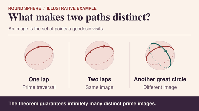
Theorem 1.1 of the original preprint says that for every integer and every smooth Riemannian metric on the standard smooth sphere , there are infinitely many prime closed geodesics with pairwise distinct images.
Prime means traversed once, over the least positive period. An image is the set of points visited along that trajectory. Start at another point on the equator, reverse direction, or go around twice, and the image is still the same. A prime trajectory can also cross itself if it passes through a point with two different velocity directions. Simplicity rules out such crossings, so the theorem counts prime images whether or not they are simple.
4. Why Classical Methods Could Not Settle Higher-Dimensional Spheres
Birkhoff’s minimax argument searches a family of loops for a bottleneck that loop shortening cannot push away. Lyusternik and Fet established the existence of a nonconstant closed geodesic on closed positive-dimensional Riemannian manifolds. Infinitude presents a different counting problem. Even a single periodic orbit produces infinitely many critical loops by iteration.
Gromoll and Meyer showed that unbounded free-loop-space Betti numbers over a field force infinitely many geometrically distinct closed geodesics on a simply connected closed manifold. Betti numbers measure the number of independent homology classes in each degree. Sphere loop spaces have bounded ranks degree by degree, so the criterion runs out of leverage. For the two-sphere, Bangert’s work together with Franks’s or Hingston’s gives infinitude by other means. Rademacher obtained infinitude for generic strongly bumpy metrics on compact simply connected manifolds. In the limit to an arbitrary metric, distinct prime images can cease to be distinguishable, so approximation alone gives no infinitude theorem.
5. The Complete Proof Strategy in Six Stages
OpenAI’s release attributes the results to an internal frontier model. The manuscript’s proof and public source files give the logical sequence below. The repository’s published reasoning summaries cover other results in the release.
- Assume finitely many images. Each nonconstant periodic loop must then come from repeating one of a finite list of prime trajectories.
- Control the repeats. Limit how much local topology each iterate can contribute and identify the cohomological degrees it can reach.
- Bound the cost of filling. Show that any ordinary cycle that eventually bounds already bounds after one fixed increase in the energy cutoff.
- Compute the global symmetry classes. Use the round metric to find paired classes in the full loop space and carry the classes over to the arbitrary metric’s filtration.
- Bound the extra classes and apply doubling. Rule out long strings of temporary classes, then use twice-traversed loops to compare the numbers at two cutoffs.
- Force an unpaired first appearance. Doubling at a maximal count requires an odd-stage class to be accompanied by its partner. At its first appearance the local geometry prevents that pairing.
6. Free Loop Spaces, Energy and the Finite-Geodesic Assumption
The free loop space contains period-one loops of Sobolev class . These loops have square-integrable velocity and no prescribed starting point. The constant loops form a copy of the sphere, denoted . For a loop , the proof uses energy and the sublevel defined by its square root . Square-root energy bounds length above by Cauchy–Schwarz and equals length at constant speed. The critical points of energy are constants and smooth closed geodesics.
Suppose prime has length . Its th iterate has length and Morse index , which counts independent directions that lower energy to second order. Bott-style iteration estimates keep the index within a fixed distance of , where is the limiting index per traversal. Thus the iterates lie near a line in the plane of length and index. Zero mean index is allowed and keeps all the corresponding indices in a bounded range.
Degenerate iterates have additional zero directions beyond the change of starting time. Theorem 3.7 controls their local homology by reducing the possible kernels to finitely many root types of the linearized return map. The local ranks stay uniformly bounded, concentrated in degrees near each iterate’s index. A common descending flow also makes the local comparison maps compatible with the half-period symmetry. Both controls matter when counting what can change as a cutoff passes a critical value.
7. The Uniform Filling Theorem and Filtered Cut–Join Identity
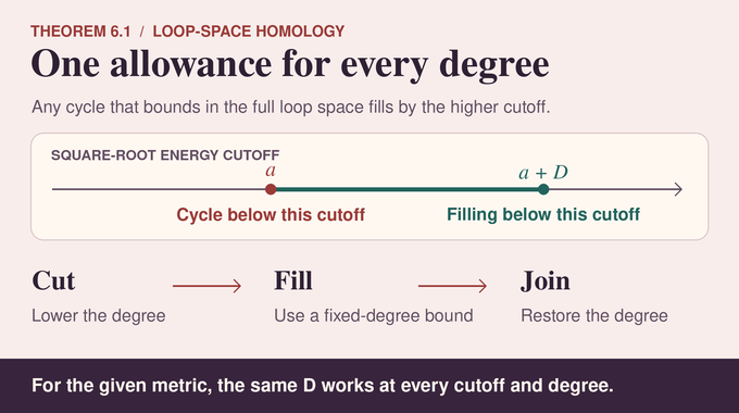
A null-homologous cycle is a family of loops that bounds a chain in the full space. Its filling may initially involve much longer loops. Fixed-degree shortening controls the extra length, but delivers a different bound for each homological degree. Theorem 6.1 gives a single increment . A cycle below that bounds globally already bounds below , both absolutely and relative to constant loops. The result holds over and requires no assumption of finitely many geodesics.
The proof first works with length. A cohomology power selects cuts at returns to a loop’s basepoint and forces the discarded piece to consume a minimum length. This lowers a high-degree cycle to a degree between two and , where the fixed-degree estimates suffice. The loop product joins compatible loop families and restores the original degree using a complementary homology power.
Why does the rebuilt filling stay short? Hingston and Rademacher’s length resonance makes the cut’s minimum discarded length and the restoring power’s length threshold differ by a bounded amount. The filtered cut–join identity lets the proof transfer the cut to the restoring power, where it returns the constant-loop fundamental class in homology, the unit for the loop product. This identifies the reconstructed boundary with the original cycle while keeping one uniform length allowance. Reparametrizing by arclength transfers the estimate to square-root energy.
8. Reflection Symmetry and Global Equivariant Cohomology
Loop reversal exchanges the two directions of traversal. Half-period translation fixes exactly the double loops, which are of the form . For example, an equator covered twice in one unit of time has twice the velocity magnitude of a single traversal, so its square-root energy doubles. The fixed part of the sublevel at therefore identifies with the sublevel at by taking the half-length root.
Let be reflection-equivariant cohomology below , relative to the constants, with mod-two coefficients. Equivariant cohomology tracks the topology together with the group action. The full-space group is . Theorem 7.2 computes a basis by first using the round metric, where geodesics of a given traversal number form a critical manifold. Gysin exact sequences relate the cohomology for the full reparametrization group to that for its subgroups.
Each round-filtration stage supplies bottom classes and partner classes. A partner is the cup product of its bottom with , the pullback of the sphere’s top cohomology class by evaluation at time zero. This operation raises degree by . The pairs are global classes, but their restrictions to an arbitrary metric’s sublevels may appear at different cutoffs. Odd here means an odd traversal number in the round filtration. The full-group lifts of odd-stage bottom classes supply the extra constraint used at equality in the doubling step.
9. Controlling Transient Classes: A Linear Versus Quadratic Conflict
Some reflection classes at cutoff do not come from the full loop space. Let count their total dimension across degrees, the dimension of the cokernel of the restriction . Under the finite-prime assumption, the index estimates and the filling increment confine possible changes in ordinary cohomology to fixed-width bands in degree, centered on lines proportional to the cutoff. Global length resonance adds another such band. In the gaps, multiplication by the degree-one reflection class identifies consecutive transient groups. One extra class in a long gap would therefore generate classes in linearly many degrees.
The finite-cut comparison in Theorem 8.2 measures the mismatch between actual equivariant degrees at and root degrees on its half-translation fixed locus. The summed defect is because linearly many iterate labels contribute to only a bounded number of degree comparisons each. From a long string, the proof lifts linearly many independent classes and shifts their root degrees to make them register as defects at linearly many cutoffs. That would yield , impossible for large . The remaining bands have bounded width, and local rank estimates together with the uniform filling bound in low degrees give a uniform bound on .
10. Loop Doubling and the Contradiction That Forces Infinitely Many Geodesics
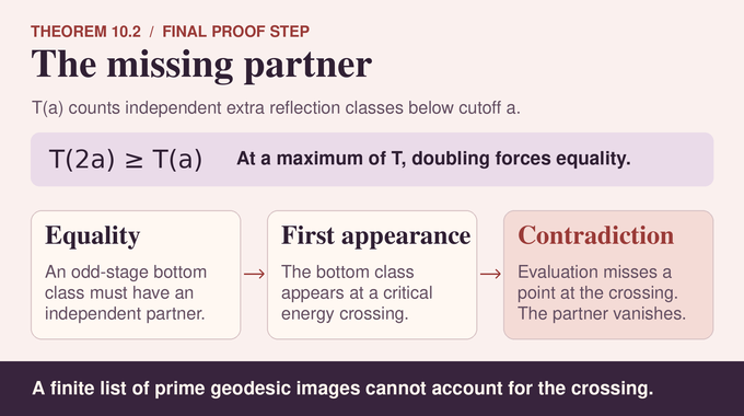
The full-group Gysin sequences split the total reflection rank at into the rank at and an even contribution from equivariant torsion. Subtracting the global-image ranks gives Theorem 10.2’s inequality at every positive regular cutoff .
When equality holds, every odd-stage bottom that restricts nontrivially at must have a partner independent of all bottom restrictions in the partner’s degree. Since is a bounded integer on regular cuts and stays constant between critical values, it attains its maximum on an open interval of regular cuts. Repeated doubling propagates that maximum to every regular point of the expanded intervals, where the equality rule applies.
The resonance threshold advances linearly in degree as the cutoff rises. Odd-stage bottom degrees have fixed spacing, so a wide expanded interval sweeps past one outside the exceptional bands at both endpoints. That bottom vanishes near the lower end and is visible near the upper end. Take its first activation. Its new restriction comes from the local cohomology of the critical crossing. Evaluation there avoids a point outside the finite union of prime images. The punctured sphere has zero top cohomology, so cup product with vanishes on the crossing. The bottom is visible while its partner is zero, violating the equality rule. This rules out a finite list of prime images.
11. Beyond Spheres: The Result for Every Closed Three-Manifold
Pull a metric back along a finite spherical cover and the projection becomes a local isometry. Geodesics upstairs project to geodesics downstairs. For a cover of degree , at most prime images upstairs can project to one image downstairs. To see why, fix an oriented parametrization of the downstairs geodesic and a point on it. Each of the points over that start determines one lift. Going around once permutes the fiber, so each lift closes after finitely many circuits. Infinitely many upstairs images therefore force infinitely many downstairs, including on real projective spaces of dimension at least two.
For a connected closed three-manifold with finite fundamental group, the elliptization case of Perelman’s geometrization theorem supplies a finite spherical cover. For infinite fundamental group, the theorem of Rademacher and Taimanov supplies infinitely many distinct images directly for the given metric. These cases also cover nonorientable manifolds. On a disconnected closed three-manifold, the result applies to each connected component.
12. What OpenAI’s Proof Establishes and What Remains Open
The preprint establishes an existence theorem for arbitrary smooth Riemannian metrics in its stated settings, including metrics with degenerate closed geodesics. It gives no general algorithm for enumerating the prime images of a given metric. Infinitely many images can share a length, as all great circles on the unit round sphere have length . The general question for closed Riemannian manifolds of dimension four and higher remains open outside settings where infinitude is known. OpenAI’s public Lean manifest lists formalizations for other results in the collection. Family 345, which contains this preprint, is absent from that list.
A geodesic on a sphere depends on the metric even though the infinitude of distinct closed images survives every smooth choice of metric. With a finite list of prime paths, doubling would require a global class to acquire a partner at a crossing where that partner must vanish. Follow Binary Verse AI for more research explainers on geometry and dynamics, from the Cartan–Hadamard conjecture to chaos in the standard map.
What are the geodesics of a sphere?
On a standard round sphere, geodesics are arcs of great circles. Every nonconstant geodesic, when continued indefinitely, traces a great circle and returns to its initial position and heading. On a sphere with an arbitrary Riemannian metric, individual geodesics can take other shapes or fail to close.
Why are geodesics on a round sphere great circles?
A geodesic has zero intrinsic acceleration. On a round sphere, its acceleration in the surrounding Euclidean space is therefore normal to the sphere. The motion stays in the plane through the center spanned by the initial position and velocity. That plane cuts the sphere in a great circle.
What is the geodesic equation?
In local coordinates, it is . The Christoffel symbols are determined by the metric, and the repeated indices are summed. The equation expresses zero covariant acceleration.
Does every distorted sphere have infinitely many closed geodesics?
Yes. OpenAI’s Theorem 1.1 states that every smooth Riemannian metric on the standard sphere , for , admits infinitely many prime closed geodesics with pairwise distinct images.
What is the difference between a prime and a simple closed geodesic?
A prime closed geodesic traverses its periodic trajectory once, over its least positive period. A simple closed geodesic has no self-intersections. A prime closed geodesic can intersect itself.
What is new about OpenAI’s closed geodesic proof?
Infinitely many closed geodesics on the two-sphere were already known. The preprint proves infinitude in every higher sphere dimension for arbitrary smooth Riemannian metrics, including metrics with degenerate closed geodesics.
Does OpenAI’s proof apply to every Riemannian manifold?
The theorem covers spheres, closed manifolds admitting a finite smooth spherical cover, and every nonempty closed smooth three-manifold. Infinitude for arbitrary closed Riemannian manifolds in dimensions four and higher remains open in general.