

Apply OpenAI’s operator to a vector supported at coordinates 0, 1, 2, and onward, and its support stays in that same tail. Now apply a second operator that commutes with the first. Even a vector concentrated at coordinate 0 can land at coordinate −1, in a different fiber. That backward move is the mechanism behind a negative answer to the hyperinvariant subspace problem. OpenAI constructs a nonzero quasinilpotent operator on a separable complex Hilbert space that has many ordinary invariant subspaces but no nonzero proper closed subspace invariant under its entire commutant.
Table of Contents
1. What OpenAI’s Proof Establishes About the Hyperinvariant Subspace Problem
Theorem 1.1 of Backward Intertwiners and a Transitive Commutant builds a bounded operator out of a measurable family of bilateral weighted shifts. Each fiber has exactly the coordinate tails as closed invariant subspaces. A contraction couples successive fibers and sends each tail with a finite cutoff densely into the preceding tail. The shift, the intertwiner, and the scalar multipliers generate a transitive algebra. An algebra is transitive when its only closed common invariant subspaces are zero and the whole space.
| Topic | Result |
|---|---|
| Question | Does a bounded nonscalar operator always have a nonzero proper closed hyperinvariant subspace? |
| Answer and Scope | No. Corollary 1.2 gives a counterexample on every infinite-dimensional separable complex Hilbert space. |
| Forward Operator | A nonzero bilateral weighted shift acting fiber by fiber, with operator norm and spectral radius zero. |
| Backward Intertwiner | A commuting contraction that transports vectors to the next base point and moves their coordinate indices down by one. |
| Commutant | A proper, strongly closed, unital transitive algebra. Its only common closed invariant subspaces are zero and the entire Hilbert space. |
| Ordinary Invariance | Each fixed coordinate tail remains a proper closed invariant subspace for the forward operator. |
Corollary 1.2 transfers the example to every infinite-dimensional separable complex Hilbert space by unitary equivalence. The commutant is proper and strongly closed, so this example also answers negatively the question of whether every unital transitive operator algebra is strongly dense in the algebra of all bounded operators. The paper is part of OpenAI’s mathematics release. The family-293 Lean scope note documents the existence theorem with the stated commutant properties.
2. Invariant vs. Hyperinvariant Subspaces: What Was the Original Problem?
For a bounded operator on a complex Hilbert space , a closed subspace is invariant if . Hyperinvariance requires for every in the commutant of an operator. Writing for the bounded linear operators on , the commutant is
The problem asks whether every bounded nonscalar operator on an infinite-dimensional separable complex Hilbert space has a nonzero proper closed hyperinvariant subspace. Since belongs to its own commutant, hyperinvariance implies ordinary invariance. The ordinary invariant subspace problem asks only for a subspace preserved by . Here the fixed tails supply such subspaces explicitly. The counterexample addresses what can be guaranteed about the whole commutant.
The distinction also explains why adjoints matter. In a self-adjoint algebra, common invariant subspaces are reducing, meaning their orthogonal complements are invariant too. The associated projections then commute with the algebra. This is the setting of irreducible representations of C*-algebras. Here the stronger test for a candidate subspace is invariance under an algebra that can contain operators without containing their adjoints, so the projection argument applies first to the self-adjoint multiplier family.
3. Why Earlier Weighted-Shift and Operator-Algebra Methods Were Insufficient
Domar’s weighted-translation theory supplies the support-separation method. Grabiner’s work on unicellular shifts gives the setting in which the invariant subspaces form a chain. Classifying a shift’s invariant subspaces narrows the possibilities for hyperinvariance, but the classification alone leaves open how other commuting operators act on the chain. The missing step in this construction is a bounded commuting map that changes the cutoff between fibers.
Arveson’s density theorem gives a strong positive result under an extra hypothesis. A transitive algebra on a separable Hilbert space is strongly dense if it contains a maximal abelian self-adjoint subalgebra of all bounded operators. The scalar multipliers here leave an entire infinite-dimensional coordinate space at each base point. For example, the projection onto coordinate zero commutes with them, although a scalar multiplier acts identically on all coordinates at that point. Thus the multiplier algebra used in the proof falls outside Arveson’s hypothesis.
The manuscript contrasts its construction with Atzmon and Sodin’s completely indecomposable bilateral weighted shifts, whose spectrum is the unit circle. Their invariant-subspace analysis left open the hyperinvariant question for those shifts. OpenAI’s added base variable gives it room to design a different commuting action. It also describes a companion construction with an irrational rotation on the circle. The 2-adic proof supplies the concrete coordinate lattice and explicit power estimate developed below.
4. Constructing the Weighted-Shift Operator on a Hilbert Space
Let , the square-summable sequences indexed by all integers, and let be the unit vector at coordinate . For a finite integer , the tail is the closed span of the with . The label gives the whole fiber and gives the zero space. On the base with probability measure , the global Hilbert space is , the space of square-integrable vector fields.
Here is the weight attached to the step from to . For instance, in becomes . The indices advance, so the image lies in and hence in . This explains why tails are invariant. Determining whether other subspaces can survive the shift requires controlling vectors with contributions at arbitrarily distant coordinates.
5. The Quadratic Weighted-Translation Criterion: Why Only Coordinate Tails Survive
Lemma 2.1 rewrites a fiber as a right translation on sequences with norm given by the square sum of , where is positive and decreasing. The map is unitary onto and carries to the shift with weights . Convexity of on the nonpositive indices means successive differences increase. They decrease on the nonnegative indices, where the logarithm is concave. The lemma also needs the signed-root sum to be finite, and the following growth for some .
Take a vector in a proper closed invariant subspace and a nonzero continuous linear functional represented by coefficients that annihilates the subspace. Their correlations vanish at every nonnegative shift . For example, if starts at and the last nonzero entry of is at , the shift aligns those endpoints. The sum has just one possible nonzero term, the product . That makes vanishing impossible. The proof bounds coefficients at the relevant end by a convex envelope of negative log magnitudes whenever its support extends indefinitely in the relevant direction. Where the envelope bends strictly it touches an actual coefficient. If both problematic ends are unbounded, the proof matches slopes at two such contact points. Their product dominates the other middle terms by geometric decay, with relative sum at most for . Normalized estimates make the two outer tails negligible. That correlation therefore cannot vanish.
The resulting support separation places each annihilator’s rightmost index at or before the vector’s first supported index. The zero-shift pairing rules out equality. Once the earliest index attained by any vector in the subspace is identified, every vector vanishes below it and every annihilator vanishes on its tail. Closedness and separation by continuous functionals give exactly that tail.
6. How 2-Adic Weights Produce the Required Opposite Drifts
The base is , the 2-adic integers, whose points record compatible residues modulo every power of two. Put and let be the residue between zero and . Under Haar probability every residue at level has mass . The map permutes these residues cyclically. An invariant set has the same conditional proportion in each residue class. Since those classes generate the measurable sets up to completion, the invariant set is independent of itself, giving ergodicity.
Write and uses blocks with and . For , the formula below uses , , and . The positive side uses for and the negative side uses for . Both central exponents equal .
Advancing the base usually raises the positive exponent by and lowers the negative exponent by . A residue wrap reverses those increments in that block. For example, at level two a move from residue 1 to 2 gives changes of and . A move from 3 to 0 gives and . Across block boundaries the offsets keep both side sequences increasing outward. Their corrections are uniformly , so cumulative log weights have quadratic limits with . The bound also gives the signed-root summability, completing the hypotheses in every fiber.
7. The Explicit Power Bound That Proves Quasinilpotence
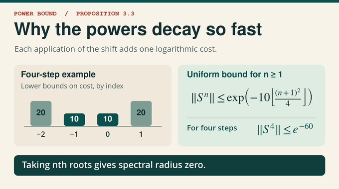
A power multiplies a basis vector by the product of consecutive weights before shifting it by indices. The logarithmic cost per step is at least , with for and for . The cheapest interval centers as closely as possible on indices −1 and 0, where both costs have . For the minimum sum is . For it is . Each fiber power sends different basis vectors to orthogonal outputs, so the bound on products is a norm bound. Its uniformity in gives the same estimate on .
For four steps the lower costs are , yielding the upper bound . These are lower bounds on the logarithmic costs, since the residue terms can increase the actual costs. For two steps, the interval at −1 and 0 uses the two exact central weights, so . This gives a case of equality. Taking th roots makes the bound tend to zero because the floor term grows quadratically. The spectral radius formula therefore gives radius zero. The two central weights are exactly , so this is the exact operator norm.
8. The Backward Intertwiner: Building an Operator That Commutes but Moves Tails
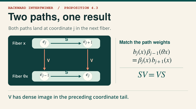
Define with . Both orders of composition starting at in fiber end at coordinate in fiber . Equating the coefficients gives the recurrence. Since every shift weight is positive, it can be solved in both directions starting from . For the central input index , the two weights in the recurrence are both , so . At other indices the ratio compensates for both the coordinate change and the change of base point.
A wrap at level has probability . The sum over levels is finite, so the first Borel–Cantelli lemma leaves only finitely many exceptional blocks almost everywhere, even with dependent levels. In the logarithm of the unnormalized coefficient, the forward sum takes the negative of the cumulative positive-side drift, and the backward sum takes the cumulative negative-side drift. Beyond the finitely many exceptional blocks, each contributes times the distance from zero plus a finite fiber-dependent additive constant. Telescoping introduces a boundary term with linear slope and a sublinear correction. Since , the unnormalized coefficients tend to zero at both ends.
A countable supremum of these coefficients is measurable and finite on the invariant set of full measure obtained by taking all translates of the good set. Dividing by that supremum leaves the recurrence intact and makes the fiber maps contractions. Setting the coefficients to zero off that set and using probability preservation yields a global contraction with . Every basis direction in is attained from where the coefficients are positive. Taking closures gives . The coefficients decay to zero, so the argument uses density, with no surjectivity assumption.
9. From Scalar Multipliers to Measurable Fields of Invariant Subspaces
Suppose a closed subspace is invariant under , , and every scalar multiplier , defined by for essentially bounded . The family contains adjoints, since . Therefore reduces each multiplier and its orthogonal projection commutes with them. The field lemma gives a measurable projection field with . Membership in becomes a pointwise condition almost everywhere.
Testing the invariance identities on constant basis fields yields fiber invariance under and transport of into under . Countably many basis tests suffice. The first condition makes . The label is measurable because holds precisely when .
10. The Decisive Contradiction: Why Strict Descent Forces a Transitive Commutant
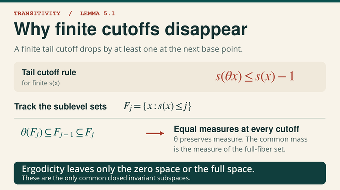
A finite input label forces the next fiber to contain the closed tail starting one coordinate earlier. Tail inclusion reverses the order of labels, giving
A full input fiber also forces a full output fiber by density. In Lemma 5.1 let and . Up to null sets, , so probability preservation makes invariant modulo null sets. Ergodicity gives it measure zero or one. Also , so all the have equal measure. Their intersection over all integer cutoffs is . If is null, each is null, and their countable union excludes finite labels almost everywhere. The argument compares the measures of nested sublevel sets, so it works even if the labels have no finite expectation. Only the all-zero and all-full fields remain. The generated algebra is transitive, and the full commutant inherits that property because it contains the generators.
11. What the Counterexample Changes and What It Leaves Open
Commutation is preserved under strong operator limits, which converge in norm on each vector. The coordinate-zero projection fails to commute with on the constant field , so the commutant is a proper strongly closed transitive operator algebra. Each ordinary fixed tail survives and loses invariance under . Each fiber shift is compact by truncating its decaying weights. Globally, an orthonormal sequence of scalar functions at coordinate zero moves to an orthogonal sequence at coordinate one with common positive norm . Hence the global operator is noncompact.
There is a second structural distinction in Section 6.3. Let be the unweighted forward shift and . Each polar conjugate reads one shifted weight. A finite family gives a countable partition into joint value sets, producing an atomic abelian von Neumann algebra. The whole family recovers both the coordinate, from the two central weights, and every 2-adic residue. It generates the diffuse multiplication algebra on . The modulus has pure-point spectral resolution, while the combined family distinguishes arbitrarily fine residue classes of a nonatomic base. This diffuse algebra sits outside the commutant: the modulus scales coordinates zero and one differently, while the shift sends the former to the latter. The spectral calculation is independent of the transitivity argument.
The answer to the hyperinvariant subspace problem rests on the interaction between the fiber classification and the commuting transport. Even an explicit chain of ordinary invariant tails can leave the commutant with no common nontrivial closed subspace. Follow Binary Verse AI for more research explainers in operator theory, from the Crouzeix conjecture on the numerical range to the Phillips–Toms formula, and for coverage of machine-checked mathematics.
What is the hyperinvariant subspace problem?
It asks whether every bounded nonscalar operator on an infinite-dimensional separable complex Hilbert space has a nonzero proper closed subspace invariant under every bounded operator commuting with it. OpenAI’s construction gives a negative answer.
Did OpenAI’s proof solve the ordinary invariant subspace problem?
No. The constructed operator preserves every fixed coordinate tail. The proof shows that its commutant has no nonzero proper closed common invariant subspace.
Why is the constructed operator quasinilpotent?
The paper bounds the norm of the nth power by an exponential whose exponent is negative and has quadratic growth in magnitude. The nth root of that bound tends to zero, so the operator has spectral radius zero.
What is a backward intertwiner, and why is it essential?
It is a bounded operator that commutes with the constructed shift and moves coordinate tails backward between fibers. Its image of a tail is dense in the preceding tail, so common invariance forces the next fiber to contain that larger tail.
How does the proof establish a transitive commutant?
The only closed subspaces simultaneously invariant under the shift, the backward intertwiner, and every scalar multiplier are zero and the full Hilbert space. Each of these generators belongs to the shift’s commutant, so the same conclusion holds for the full commutant.
Why does the result not contradict Arveson’s density theorem?
Arveson’s theorem requires the transitive algebra to contain a maximal abelian self-adjoint subalgebra. The scalar multiplier algebra used here has infinite multiplicity and fails maximality. The projection onto a single coordinate commutes with every scalar multiplier and lies outside their algebra.
What part of OpenAI’s proof is documented in Lean?
OpenAI’s family-293 Lean documentation records the existence, on every infinite-dimensional separable complex Hilbert space, of a nonzero quasinilpotent operator with a proper, strongly closed, transitive commutant. The scope note states the existence theorem without itemizing every intermediate step of the manuscript.