
A floor tiled with squares uses one square’s worth of material per square’s worth of space. In high dimensions, some convex shapes make that economy impossible even when you can place each copy wherever you like. OpenAI’s September 2026 preprint proves that, in every sufficiently large dimension, some centrally symmetric convex body has translative covering density greater than for an absolute constant . Combined with Rogers’ upper bound, that puts the worst-case covering density of convex bodies at order . The decisive step is to find a single body that defeats every low-density placement, including placements designed after its shape is known.
Table of Contents
1. What Is Translative Covering Density, and How Is It Measured?
A convex body in is compact, contains the segment between any two of its points, and has nonempty interior. A translate moves every point of the body by the same vector , preserving its orientation and size. A set of centers covers space if every point belongs to at least one of those translates. The paper takes to be locally finite, so each bounded region contains finitely many centers.
| Quantity | What It Means |
|---|---|
| Setting | Translated copies of one convex body cover all of Euclidean space. |
| Density | The volume of the copies per unit volume, counting overlap. |
| Hard Examples | Some centrally symmetric bodies exceed in every sufficiently large dimension. |
| Worst-Case Order | Rogers’ upper bound and the new examples give . |
The paper measures an arrangement using the number of centers in the cube . Multiply the count per unit volume by , take the upper limit as the cube grows, and then take the infimum over covering arrangements. The upper limit allows for arrangements whose center counts per unit volume never settle to a single value.
For a periodic covering, a full-rank lattice repeats a finite set of distinct offsets modulo the lattice. Each offset produces one copy of the lattice, called a coset. The periodic density is , where is the volume of a fundamental cell. This density equals the average number of translates containing a point in that cell. A lattice covering uses just one coset. The planar triangular lattice illustrates that a lattice basis can use nonperpendicular vectors, so its fundamental cell can be skewed.
For a worked example, unit squares centered on give a periodic tiling of the plane with density 1. Place the same squares on a square grid spaced half a unit apart in both directions. Each cell now has area , so the density is 4 and almost every point lies in four squares. Both arrangements cover the entire plane. The extra density records the repeated coverage.
2. Rogers’ Covering Bound and the Unresolved Linear Question
In 1957, C. A. Rogers showed that every convex body in dimension admits a periodic translative covering with density at most
Here and throughout the paper, is the natural logarithm. Gábor Fejes Tóth later improved the lower-order term and obtained coverings using only cosets.
Equal Euclidean balls were known to force a density at least proportional to dimension. That lower bound left room for a single constant times dimension to cover every body. Márton Naszódi recorded that universal linear-bound question, which the new manuscript answers.
3. OpenAI’s Theorem: Some Symmetric Convex Bodies Require n log n
Theorem 1.1 says that there are absolute constants and such that for every integer there exists a centrally symmetric body satisfying
Here is the optimal translative covering density. Reflection through its center leaves a centrally symmetric body unchanged. The body can vary with dimension. For any proposed universal bound , taking sufficiently large makes exceed . There is then a symmetric counterexample in that dimension. Rogers’ bound and the theorem put the supremum of between positive constant multiples of , even when the supremum ranges only over centrally symmetric convex bodies.
4. Why Earlier Lattice Covering Proofs Could Not Settle the Problem
Heng Li and Xizhi Liu had already proved an order- lower bound for lattice covering density. Their random-slab construction supplied much of the geometric and probabilistic machinery used here. The restriction to one lattice matters because an optimizer with several offsets can interleave separate copies of the same grid. A lower bound on each single-lattice covering gives no lower bound of the same size on the optimum over all these additional choices.
There is also a difference between randomizing centers and randomizing the body. In the packing-torus model studied by Bukh and coauthors, Poisson centers can fail with high probability at a specified density of order . A specially placed set of centers might still cover that given body. OpenAI instead samples a body and needs one outcome that defeats every permitted low-density arrangement.
5. Constructing the Difficult Convex Body Using Random Slabs
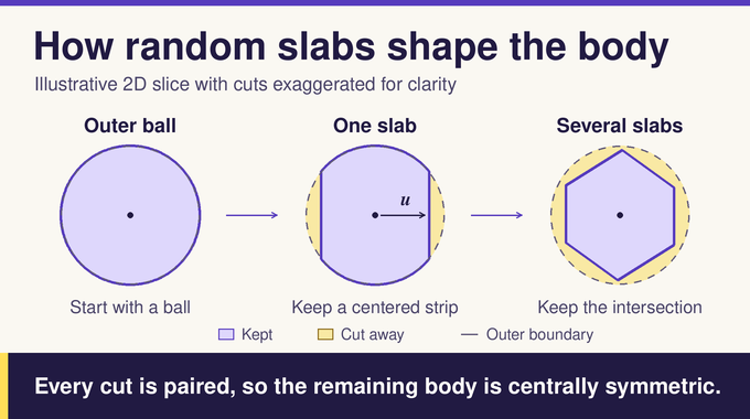
Start with the Euclidean unit ball . Set and , and take an outer ball of radius . A unit vector specifies a slab of half-width 1 around the origin. Let be a Poisson process on the unit sphere with intensity measure , where is uniform probability measure on the sphere. Equivalently, draw a Poisson number of normals with mean , then choose each independently and uniformly. The body is
Every slab and the outer ball are symmetric about the origin, and their intersection contains . The parameter is the reciprocal of the surface probability that a normal cuts a point at distance . At distance at most , the expected number of cutting normals is at most 1, so the probability a point survives is at least .
Integrating this survival probability over gives expected volume at least , where . The outer ball caps the volume at less than . Lemma 2.1 combines these bounds to give a dimension-independent positive probability of volume strictly greater than , with . That margin later converts a bound on centers per unit volume into a bound on covering density.
6. Reducing Infinitely Many Covering Arrangements to Finite Patterns
Proposition 3.1 starts from a hypothetical periodic covering at or below a fixed center-intensity threshold. Averaging modulo its lattice gives the expected number of indexed centers in a shifted window as intensity times window volume. The calculation works for short periods, skew fundamental cells, and any finite number of cosets. Every occurrence contributes to the average, including repeated center positions in an indexed list.
The proof picks a translate of a small ball , of fixed radius , with two properties. Its neighborhood has few enough centers to retain in a bounded list, and a substantial fraction of points in the window are suitable targets. Those targets have no center extremely close by, only a controlled number of centers within covering distance, and bounded total radial cost. The last condition sums the weights over nearby centers, with the distance to the target. The weight rises as a center moves inward from distance . Average estimates and Markov’s inequality give a window where these requirements coexist.
Each retained center is rounded to a fixed grid. Two indices that round to the same point are kept, so the count and cost estimates still apply to the full list. The displacement is absorbed by a slightly enlarged body , obtained by adding to both the ball radius and the slab half-width, with . Coverage of the original window by therefore implies coverage of by the rounded translates of .
This produces a finite family of possible lists before the normals are drawn. The logarithm of the number of lists is at most , where . Any covering at the specified intensity must leave a pattern in this family.
7. Spherical Caps: How a Slab Creates an Uncovered Point
At a target , only a center within the outer radius of can contribute coverage. Its residual vector is . The normals that cut this residual form an antipodal pair of spherical caps:
Indeed, if belongs to , the residual violates the slab constraint, so falls outside . For a residual of length , a half-cap consists of directions within angle of its signed axis when . Longer residuals give wider caps at the same threshold. This explains the radial budget: shorter residuals generally require rarer normals and cost more in the estimate.
Two cap pairs can share candidate normals. The natural angular distance is the smaller angle between their axes after identifying opposite directions. The paper bounds normalized cap overlap by a quantity that falls exponentially with a distance combining angular separation and the difference in logarithmic cap intensities. It also lower-bounds the common intersection for suitably clustered caps. Together these estimates say when several cuts can share a normal and when sharing is unlikely.
8. Grouping Cap Conditions and Building Poisson Witnesses
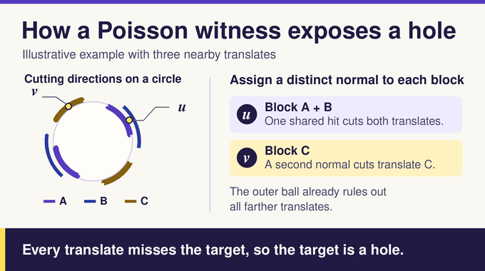
Requiring an independent cut for each residual would misrepresent nearly coincident caps. The proof groups the residual indices into blocks and chooses one measurable subset of the common cap intersection for each block. A normal in that subset cuts every translate in its block. For example, if three center indices coincide after rounding, their three cap conditions are identical. A single normal in that common cap cuts all three occurrences.
A witness assigns a distinct sampled Poisson point to each block’s subset. This is a sufficient certificate of a hole: all nearby translates are cut, and farther translates were already ruled out by the outer radius. For labeled blocks the expected number of such assignments, called the activity, is the product of their subset intensities. The Poisson factorial-moment formula gives that product even when subsets overlap.
The partition must keep the activity large enough and control how assignments can overlap. Proposition 5.1 merges blocks under a logarithmic cost budget. Once merging stops, its estimates bound both the total loss in subset intensities and the overlap between different subsets. Those bounds matter even at one target, where different witnesses can reuse some of the same Poisson points.
9. Janson’s Inequality and the Probability of Unavoidable Holes
For one fixed pattern, the proof selects suitable targets before sampling the normals. It uses two angular scales for residuals at different targets, with a fixed positive constant.
| Scale | Role in the Proof |
|---|---|
| Fine | Every pair of distinct targets meets this separation across all relevant residuals. |
| Coarse | Most pairs meet this stronger separation, making their cutting caps disjoint across targets. |
The selection is possible because near-parallel residuals confine the second target to a thin cylinder around an axis through its center. The cylinder’s cross-sectional volume falls rapidly in high dimension. A counting argument over the center labels and target pairs gives separation at the fine scale everywhere, and at the coarse scale for all but an exponentially small fraction of pairs.
To use Janson’s inequality, the proof compares witnesses with similar expected counts, keeping a bin in which the activities differ by at most a factor of two. An overlap diagram is a partial matching of blocks whose slots reuse the same Poisson point in two assignments. Its weight involves the measures of the shared subsets’ intersections. The sum includes same-target and cross-target diagrams.
Proposition 6.2 bounds the probability that every chosen target has zero witnesses. Write for the witness count at target , for its activity, and for the sum of nonempty matching weights for targets . In the chosen bin the bound is
The many targets keep the total activity large relative to the same-target overlap terms. Fine separation limits the dependence between the remaining pairs, and coarse separation makes most cross-target diagram sums vanish. Since full coverage forces zero hole witnesses at every target, Proposition 7.3 gives a doubly exponential upper bound on one pattern’s chance of covering the window.
10. Completing the Proof: Why Every Low-Density Covering Fails
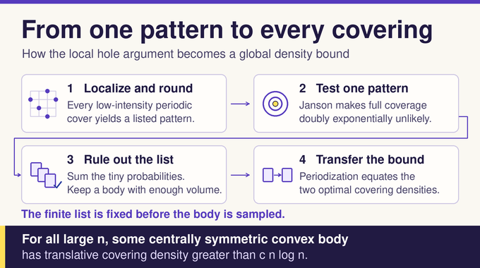
The union bound adds these success probabilities over . The fixed-pattern probability is at most , with . Its decay beats the growth in the number of patterns. Thus the probability that any retained list covers the window tends to zero. The volume event still has positive probability, so some realization has enough volume and defeats every retained pattern.
If a periodic covering of that realization had intensity at most , localization would produce a successful retained list. Hence the infimum of periodic densities is at least , which strictly exceeds by the volume margin. Appendix A gives the final transfer:
To see the principle, take a large cube and retain every center that could cover any point in it, including centers within a fixed-width border outside the cube. Repeat that finite list with the cube’s periods. In fixed dimension the relative border overhead vanishes as the cube grows, yielding equality of the two infima.
11. What the n log n Result Establishes and What Remains Open
The paper gives the same lower bound, with the same constant, for some centrally symmetric polytopes with rational vertices. Approximate the successful body from inside by such polytopes and retain enough volume to preserve the strict margin. Any covering by a smaller polytope still covers by the containing body at the same center intensity, so the same threshold applies.
A companion manuscript supplies an order- upper bound using a single lattice. OpenAI’s release announcement describes the wider collection. The family’s Lean scope note and proof code cover the order of the four suprema, for lattice and translative coverings over all convex bodies and over symmetric ones. The preprint separately supplies the written random-slab argument and rational-polytope corollary.
The construction proves existence in large dimensions. The constants are unoptimized, and the proof gives no efficiency guarantee for finding a successful body. For Euclidean balls, the manuscript records a linear lower bound in order and Dumer’s upper bound of . The exact order for that fixed shape remains open. What is settled is the worst-case translative covering density when the shape can vary. For another proof in convex geometry, read Binary Verse AI’s coverage of the logarithmic Brunn–Minkowski conjecture.
What is translative covering density?
Translative covering density is the lowest achievable density, taken as an infimum, when copies of one convex body cover Euclidean space by translations alone. Density counts the volume of the copies per unit volume of space, with overlaps counted repeatedly. It can exceed 1.
Why is n log n the optimal order for convex-body covering density?
Rogers gave a universal upper bound of order n log n. In every sufficiently large dimension, the new theorem gives a centrally symmetric convex body whose translative covering density exceeds c n log n for an absolute constant c > 0. Together these bounds give worst-case order Θ(n log n).
Why did earlier lattice covering results not solve the problem?
The earlier lower bound restricts the centers to one full-rank lattice. Allowing a periodic pattern with several lattice cosets enlarges the set of candidate arrangements. The new proof rules out every periodic pattern below its threshold and uses periodization to transfer the lower bound to unrestricted coverings.
How do random slabs and Poisson witnesses prove that coverings must have holes?
Random slabs cut a convex body out of an outer ball. At each candidate point, spherical caps identify slab normals that cut individual translates. A witness assigns distinct sampled normals to blocks of cap conditions so that every relevant translate is cut at that point. A Poisson version of Janson’s inequality bounds the probability that a pattern covers every target.
Does the n log n lower bound apply to every convex body?
The theorem guarantees difficult examples in each sufficiently large dimension. Other bodies can be much easier to cover. For example, a cube can tile Euclidean space by translations with density 1.
Does the proof settle covering density for spheres and polytopes?
It gives the same lower-bound order for some centrally symmetric polytopes with rational vertices. For Euclidean balls, the paper records a linear lower bound and an upper bound of order n log n. The exact asymptotic order for balls remains open.
How is covering density different from packing density?
Packing requires the interiors of copies to be disjoint and measures how much space they occupy. Covering requires every point to lie in at least one copy and measures the volume contributed by all copies, including overlaps.