
Give a standard Gaussian cloud as many labels as you like. For each label, add up the vectors assigned to it, weighted by Gaussian probability, and square the length of that sum. Can a fourth label, or a hundredth coordinate, improve the best total? OpenAI’s proof of the propeller conjecture gives a sharp answer. Every finite measurable partition scores at most , and three sectors already reach that value in the plane. Extending them into extra dimensions preserves the score. The central step is to show that an optimal partition cannot beat the propeller by using five or more positive-probability cells.
Table of Contents
1. What Is the Propeller Conjecture, and What Did OpenAI Prove?
Khot and Naor posed the Gaussian partition problem in their 2008 work on approximate kernel clustering. A geometric quantity controlled the Unique Games hardness analysis for a clustering problem with a fixed number of labels. Their formulation put cells in , with labels available to leave unused. They asked whether the planar propeller would still maximize the score when both the dimension and the available label count grew.
Theorem 1.1 of OpenAI’s September 24, 2026 manuscript, The Gaussian propeller bound in every dimension, proves the following for all positive integers and and every measurable partition of . Here is standard Gaussian probability measure and the norm is Euclidean.
| Feature | What the Theorem Establishes |
|---|---|
| Upper bound | for every finite measurable partition. |
| Dimension and labels | Positive integers and . Extra labels can be left empty. |
| Cell probabilities | Unrestricted. The partition is taken up to Gaussian null sets. |
| Attainment | Three planar sectors, extended orthogonally, attain the bound for and . |
The theorem proves attainment under the stated dimension and label conditions. A classification of all equality cases is a separate question. The manuscript appeared in OpenAI’s October 2026 mathematics release.
2. Gaussian First Moments: Understanding the Quantity Being Maximized
The measure has density relative to ordinary volume. A point’s contribution has a direction and a size, weighted by the Gaussian density at that point. Parts of a cell on opposite sides of the origin can cancel. A positive-probability cell that is symmetric about the origin, for instance, has zero first moment.
For positive mass, dividing by gives the conditional mean of a standard Gaussian vector in the cell. The paper calls the unnormalized vector the centroid. Thus a cell’s score is the square of its mass times the squared length of its conditional mean. This weighting matters when comparing a small tail region with a larger cell near the origin. The first moments of all cells sum to zero because the standard Gaussian has mean zero.
3. Why Three 120° Sectors Achieve Exactly 9/(8π)
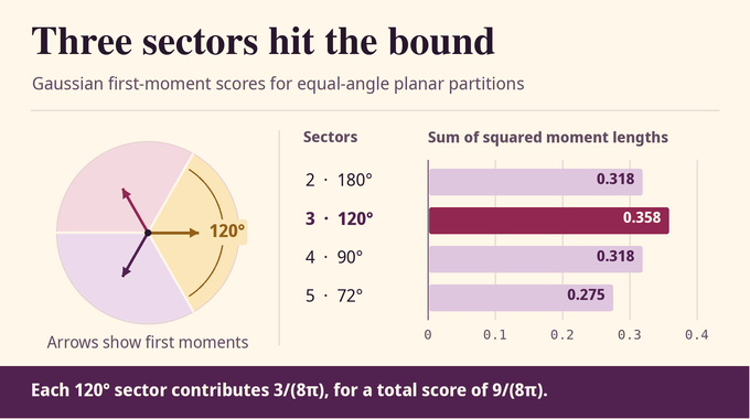
Take a planar sector with half-angle around the positive first coordinate axis. In polar coordinates, the Gaussian density contributes the exponential, while the vector and area element contribute one radial factor each. Reflection across the axis cancels the sine component. The cosine integrates to , and the radial integral equals .
The moment points along the bisector and has magnitude . For , this is . Squaring and summing three copies gives . In higher dimensions, each extra coordinate has mean zero independently of the planar sector, so the product construction leaves the three moments unchanged except for appended zero coordinates.
The same computation gives for equal-angle sectors. Two semicircles score , and four quadrants also score . Five equal sectors score , which is smaller still. These comparisons show how narrower sectors can give a lower total. The universal claim takes a different argument because a partition may use unequal angles or cells with no sector structure at all.
4. Why Earlier Proofs Could Not Settle Every Dimension
Khot and Naor determined the three-cell optimum and showed that an optimal partition can be represented by cones in the span of its centroids. Heilman, Jagannath and Naor then proved the bound for every finite partition of three-dimensional Euclidean space. Their computer-assisted proof handled the remaining four-cell conical configurations using spherical geometry and a finite verification. OpenAI takes that three-dimensional theorem as an input.
The difficulty with more labels is that an optimizer can have a larger span after the conical reduction. Four active cells suffice to span up to three dimensions at a minimum-cell optimum. Five active cells give four effective dimensions. A related route via Gaussian noise stability required an additional stability hypothesis and treated at most four cells. Noise stability measures the chance that correlated Gaussian samples share a label, whereas the propeller objective uses first moments and allows arbitrary cell probabilities.
5. How Gaussian-Maximum Duality Turns Arbitrary Partitions Into Cones
Fix an ambient dimension and a finite label budget large enough for the partition under consideration. Call the optimal score for this setting and denote the budget by . Lemma 2.1 rewrites the optimization in terms of Gaussian linear scores for a standard Gaussian in that space.
For a fixed partition, the square root of its score is the norm of the list of centroids. Euclidean norm duality expresses this norm as a maximum pairing against a list of vectors with total squared length one. Once the list is fixed, each point contributes most when assigned to the largest linear score. Ties can be broken by label order. This replaces the search over measurable assignments with a search over finite lists.
The normalized lists form a compact sphere. The expected maximum varies continuously with the list because the change in the pointwise maximum is bounded by times the largest norm of the difference between corresponding list vectors. A maximizing list therefore exists, and its score partition attains . For an optimal partition with distinct centroids, the cells agree almost everywhere with the winning-score cones defined by for every . These inequalities put the boundaries of the closed cones in score-tie hyperplanes.
6. Why Any Better Partition Must Have Five or More Active Cells
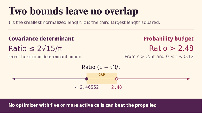
Assume the optimum exceeds and choose an optimizer with the fewest active cells, meaning cells of positive Gaussian probability. Let there be of them. Merging cells and replaces their two moments by and changes the objective by . A positive change violates optimality. A zero change gives an optimizer with fewer active cells. Every off-diagonal inner product is therefore strictly negative.
The Gram matrix of these moments has zero row sums because . Its quadratic form is a sum of positive multiples of over all distinct unordered pairs of coordinates of . Only constant vectors make every term vanish. Hence has rank , and the only dependence among the centroids is a multiple of their zero-sum relation.
Every score depends only on the projection onto their span. The orthogonal Gaussian factor again adds zero to the moments. If , the reduced partition can be placed in three dimensions with its score preserved. The earlier theorem rules out that case, so any counterexample at the optimum must have .
7. Bounding Cell Probabilities With Gaussian Rearrangement
Write for the mass of cone and for its normalized centroid length. Then . The largest of the centered scores is always nonnegative, so each winning cone lies in its score’s nonnegative halfspace and has probability at most one half.
For a fixed probability, compare a cell with the halfspace that contains the largest projections along its centroid direction. Exchanging points across the threshold can only increase the integrated projection. If the threshold is , where is the standard normal distribution function, the halfspace first moment is , with the standard normal density. This yields and a uniform lower bound on . The radius bound comes from comparing the largest possible halfspace moment, , with the square root of the assumed optimum, which exceeds . The probability bound uses the full dependence on the threshold.
When , the effective dimension is four. A cone is determined by its directions on the unit sphere , and the Gaussian radius is independent of that direction. The same comparison on the sphere uses a cap of equal directional probability. Optimizing the resulting one-variable estimates gives the following constants for the proof.
| Active Cells | Comparison Set | Mass Bound |
|---|---|---|
| Cap on | ||
| Gaussian halfspace |
8. Ehrhard’s Inequality and What Happens When One Gaussian Score Is Removed
Let and . Removing decreases the maximum on points where it wins. Recentering the remaining vectors adds the same mean-zero random score to all of them and reduces their total squared norm to . Applying the dual bound to that shorter list shows that the expected loss is at least .
The same loss is the integral over nonnegative gaps of the probability that beats every rival by at least . The score-difference normals form a basis, so a single translation of the winning cone tightens every score inequality by . Differentiating the Gaussian mass of that translate gives .
Ehrhard’s inequality makes concave in the translation parameter. The tangent at zero therefore bounds this function from above. With , the tangent has slope . Applying and integrating gives the upper bound . The slope matters because a probability measured at gap zero alone says little about how long the winning margins persist. A cell with a long centroid must contribute enough to the expected maximum that removing its score costs a definite amount. A tiny winning probability would make that loss too small. Comparing with the lower bound from recentering and using the certified interval estimates in Section 3.3 gives . For small radii, the linear term can demand much more probability than the quadratic rearrangement estimate.
9. Two Competing Scores and the Covariance Determinant
Order the radii from largest to smallest and write , , and . Project the other scores orthogonally to the direction of the smallest centroid. The Gaussian coordinate along that direction is standard normal and independent of the vector of residual scores. Two residual scores can still be correlated with each other. Their integrals over the smallest cell are zero because that cell’s centroid is orthogonal to their residual directions.
After scaling two residual scores to , winning forces and , with . The zero residual integrals let the proof replace the integral of over the cell by that of . Conditional on , taking its positive part leaves a triangle with corners , and . The affine integrand has mean height there, so the unweighted integral is .
Let be the square root of the covariance determinant for residual scores before scaling. After scaling, the density is bounded above by , where is the square root of the rescaled determinant. A larger determinant spreads out the density and lowers the upper bound on the cell’s moment. Comparing with the known moment bounds by , where the positive coefficients describe the competitors’ components along the smallest centroid and sum to one. Combining those pairwise bounds with the negative off-diagonal covariances and zero row sums gives Corollary 4.2.
10. The Final Contradiction for Five or More Cells
If the rearrangement bound uses the coefficient , the probability left after assigning the baseline to every cell totals exactly . The deletion estimate requires each cell to use at least the positive part of from that remainder.
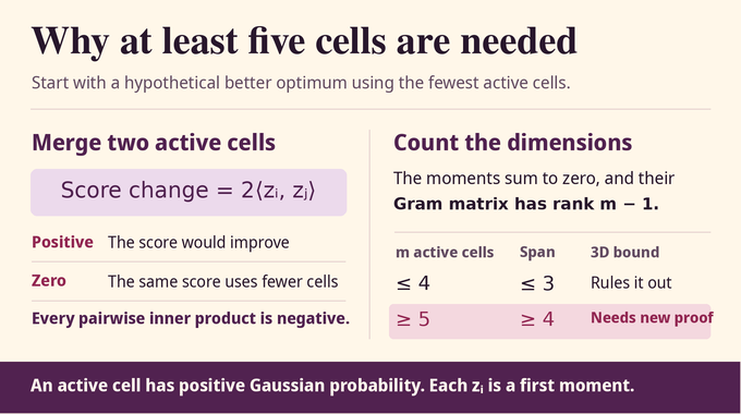
The budget first forces . Together with the first determinant inequality, it rules out . Accounting for the probability required by the smaller cells gives and then . Section 5.3 charges at least two radii beyond the first three for five cells, or at least three for six or more. If , the third radius also uses enough probability to push the total above . The argument uses concavity of to bound the charge for the third radius over the entire interval from to by the smaller endpoint charge. Even that smaller charge exceeds the available remainder once the selected smaller cells are included. This gives .
Now . The second determinant inequality would require , but the left constant is larger. Appendix A uses rational enclosures for quantities such as , square roots and Gaussian probabilities. Monotonicity or concavity makes the certified endpoint comparisons apply throughout the needed intervals. The contradiction therefore excludes the entire putative range of optimizers.
11. What the Proof Establishes for Gaussian Maxima and Kernel Clustering
For Gaussian maxima, Corollary 5.1 bounds the expected largest score by a sharp constant times the square root of the total squared length of the centered score vectors. If is their arithmetic mean, subtracting its score shifts every entry equally and leaves the expected maximum unchanged.
This also applies to a centered jointly Gaussian list with singular covariance. The planar propeller’s three centroid vectors give equality. In a list of correlated Gaussian variables , the sum inside the bound becomes . A random Gaussian component shared by every entry has no effect on this measure of spread or on the expected maximum when it has mean zero.
In Section 6, the identity-target kernel clustering problem takes a rational symmetric positive semidefinite matrix with zero row sums. It sums matrix entries over ordered pairs assigned the same label, including diagonal entries. For each fixed , Khot and Naor’s ideal Gaussian rounding with an optimal semidefinite relaxation gives an expected value of at least the optimum divided by . With their low-influence estimate and the companion Unique Games Theorem, the paper proves NP-hardness for deterministic approximation with any fixed loss factor strictly below . The endpoint guarantee uses ideal sampling. It supplies no exact finite-bit implementation or empirical clustering benchmark.
The published Lean scope covers the Gaussian moment inequality and the attaining partition. The Gaussian-maxima corollary and the clustering result sit outside that formalization. The propeller conjecture ultimately shows how two constraints on a high-dimensional optimizer, the probability its cells require and the covariance its competing scores permit, force the sharp value to remain planar. Follow Binary Verse AI for more research explainers, including the spherical perceptron in Gaussian optimization, the logarithmic Brunn–Minkowski conjecture in convex geometry, and approximation bounds for the k-median problem and edit distance.
Why are three 120° sectors optimal in the propeller conjecture?
Three equal 120° sectors attain 9/(8π). OpenAI’s proof establishes that every finite measurable Gaussian partition has a sum of squared first-moment lengths at most 9/(8π), allowing arbitrary cell probabilities and empty cells.
Could four or five sectors give a better Gaussian first-moment sum?
No. The universal bound applies to four and five sectors, including unequal angles. After the extremal reduction, the earlier three-dimensional theorem rules out an improvement with at most four active cells. OpenAI’s new estimates exclude an improvement with five or more.
Why doesn’t increasing the dimension improve the optimum?
Extending each planar sector along orthogonal directions adds only zero coordinates to its Gaussian first moment. The same construction therefore attains the bound in every dimension of at least two when at least three labels are available. The universal upper bound rules out a better score in higher dimensions.
What is the difference between a Gaussian first moment and a centroid?
The manuscript uses centroid to mean the unnormalized Gaussian first moment, the integral of the position vector over the cell with respect to Gaussian measure. Dividing that vector by the cell’s Gaussian probability gives the conditional mean when the probability is positive.
Does the proof establish that the three-sector arrangement is the only optimizer?
Theorem 1.1 establishes the sharp bound and gives an attaining three-sector construction. A complete classification of equality cases is outside that theorem’s statement.
Is the Gaussian propeller proof formally verified in Lean?
Yes. OpenAI’s published Lean formalization covers the universal bound and the construction that attains it. The paper’s separate Gaussian-maxima and kernel-clustering consequences lie outside that formalized scope.
What does the propeller conjecture prove about kernel clustering?
With Khot and Naor’s low-influence result and the companion Unique Games theorem, the bound yields NP-hardness of deterministic approximation with any fixed loss factor strictly below (8π/9)(1 − 1/k), for fixed k ≥ 3. This threshold concerns identity-target kernel clustering on rational symmetric positive semidefinite matrices with zero row sums.