
A Fourier sum can approximate a function in mean square while still behaving erratically at individual points. OpenAI’s September 23, 2026 preprint settles a sharper question about Fourier series convergence. For every complex-valued function in on the circle, the ordinary symmetric partial sums converge to the function almost everywhere along the full sequence of cutoffs. The condition admits functions outside every with . The proof gets there by controlling all cutoffs at once on most of the circle, then adding the contributions from different ranges of function values. Read the original preprint.
Table of Contents
1. What Problem Does Fourier Series Convergence Actually Ask?
| Item | Details |
|---|---|
| Paper | Almost-everywhere Fourier convergence in L log L |
| Author and date | OpenAI, September 23, 2026 |
| Input | Complex-valued functions in the circle’s L log L class |
| Output | Almost-everywhere convergence of ordinary symmetric Fourier partial sums along the full sequence |
| Proof estimate | Uniform control of the maximal partial sum on a set defined by spatial density |
Write for the circle and for its normalized length measure. The Fourier coefficient at integer frequency measures how much of the complex exponential at that frequency is present. The symmetric partial sum keeps all frequencies from through .
At a fixed point the terms have phases, and adding another pair of frequencies can undo cancellation that held at the previous cutoff. Pointwise convergence asks whether the sums settle at that point. Almost-everywhere convergence asks whether they settle outside a set of measure zero. Mean-square convergence, when available, asks whether the integral of the squared error tends to zero. Small integrated error by itself allows the locations of large errors to move with the cutoff. The paper asks whether the full sequence settles almost everywhere under the condition. For the separate computational question of evaluating finite transforms, see the discrete Fourier transform complexity proof.
2. Why Did Carleson–Hunt Stop Short of L log L?
Carleson’s theorem in 1966 gave almost-everywhere convergence for square-integrable functions. Hunt extended it to every with , the range now associated with the Carleson–Hunt theorem. At the other end, Kolmogorov’s 1923 example gave an integrable function whose Fourier series diverges almost everywhere. That leaves room for convergence guarantees strictly between the power conditions and plain integrability.
Sjölin and Antonov obtained guarantees involving extra iterated logarithms. Soria developed larger spaces by extrapolation, and Arias de Reyna’s space contains both Antonov’s class and Soria’s space. Lie proved a full-sequence maximal bound from to weak using time-frequency analysis. Di Plinio and Fragkos later obtained quantitative weak- bounds whose constants grow on the order of as approaches one. Extra logarithms impose a higher cost on large function values. The growth of the weak power-bound constants rules out a direct passage to the endpoint. The outstanding question was whether the single logarithm in suffices for every function in that class.
3. What Exactly Does OpenAI’s Fourier Series Convergence Theorem Prove?
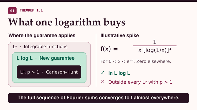
Theorem 1.1 of the preprint uses this integrability condition, with the natural logarithm.
For every complex-valued function satisfying it, one measurable set of measure zero can be excluded, after which the limit holds as runs through all nonnegative integers.
Every with is contained in here. For large , the growth of dominates , and the circle has finite measure. To see what the endpoint adds, take the following function on and set it to zero elsewhere on the circle.
Substituting turns the integral into one bounded by a constant times , which is finite. The integral instead contains , which diverges for every . The new theorem covers this spike even though every fixed power condition misses it.
OpenAI’s repository identifies the principal convergence statement as the target of the Lean formalization. That scope concerns the limit outside one null set for the full sequence. The published Lean scope and the formalization entry point identify that theorem. OpenAI also describes the broader release in its mathematics announcement.
4. Why Is the Maximal Fourier Operator So Difficult to Control?
The maximal operator looks at the largest absolute partial sum over all cutoffs, at each output point.
A bound at one cutoff leaves open what happens at every other cutoff. Even bounds of the same size for each cutoff can lose a factor proportional to the number of cutoffs if combined by a union bound. At the endpoint, that factor would defeat the summation over height layers. In the finite model the same problem reappears as a maximum over modulation frequencies and a sum along a dyadic path. The estimates must survive increasing both the frequency range and the depth of the tree.
5. What Is the Good-Set Estimate Behind the New Proof?
Start with a nonnegative density of mass one and height at most , for sufficiently large . Its uncentered Hardy–Littlewood maximal density is the supremum of the average of over circle arcs containing . Put and keep the points where is at most . Section 1.1 states the estimate proved in Theorem 10.1.
Here is an absolute constant. The spatial maximal inequality gives the discarded set measure at most . The two bounds do different jobs. For an input layer of mass , undoing the normalization multiplies the integral bound by . The discarded measure is controlled separately, by the large height parameter. Choosing layers whose heights grow doubly exponentially makes their discarded measures summable, while the integral costs fit the one logarithm in the input condition.
6. How Does the Proof Turn Fourier Sums Into a Dyadic Problem?
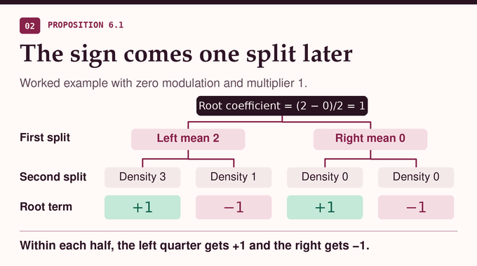
In the unit-period coordinate , modulation by integer multiplies the input by . Divide a top interval into halves, then quarters, and continue. At each node, the Haar coefficient is half the difference of the two child averages of the modulated input. On the output path, this coefficient is determined at the current node. A multiplier of modulus at most one may use the next branch choice, and the following branch provides the output sign.
In the two-level example, the four quarters have constant densities 3, 1, 0, 0. With zero modulation, the left and right half averages are 2 and 0, so the root coefficient is 1. Choose the multiplier to be 1. The delayed root contribution is then positive in the first and third quarters and negative in the second and fourth. The first branch alone would give one sign to the whole left half. This example isolates the root contribution so the extra bit is visible.
The path stops when the current average of the original density exceeds . Proposition 6.1 bounds the integral of the maximum of the stopped transforms by on a top interval of length between one-half and one and mean density at most two. Its constant is uniform in the depth and the integer modulation cutoff, and the same bound extends to the supremum over all integer modulations.
7. How Does Entropy Compression Bring Different Frequencies Into Alignment?
Lemma 3.1 begins with a finite set of integer frequencies, a bound on the size of its iterated sumsets, and a uniform bound on a noise-weighted moment of differences between two independent frequency sums. The proof then introduces correlated letters with prescribed uniform marginals. Each coordinate still samples from the same frequency set, while the joint law can exploit structure that independent sampling would miss.
Shannon entropy measures uncertainty in a discrete law. Relative entropy measures the departure of the correlated law from independent sampling, and mutual information measures what the noisy sum reveals about the letters. The proof budgets the correlation, the revealed information and the cost of the additive error together. It refines the conditional laws in two orders, then freezes contexts to find a center frequency and a retained subset.
Each retained frequency has small average phase defect relative to that center over one common region, measured under the phase distribution conditioned on that region. The lemma also bounds the loss in the logarithm of the set size. Crucially, the subset and region work for any weights subsequently put on the retained frequencies. The spectral update can therefore choose its weights after compression.
8. Why Do Thermal Labels and Spectral Updates Matter?
The proof samples an input location from the current density-weighted piece and observes the noisy label modulo one. The noise has a Gibbs-type density proportional to , where is a finite sum of cosine penalties with nonnegative coefficients.
Such noise makes some frequency characters nearly constant on the error distribution. When too many large conditional Fourier coefficients remain separated, the proof adds a spatial term and a phase penalty suggested by compression. Positivity of the Fourier coefficients and the Griffiths–Ginibre covariance argument imply that adding thermal penalties increases the normalized cosine coefficients. Hence the mean squared phase defects decrease as the form is tightened.
The update has two routes. A regular success provides evidence unlikely under the comparison law, where membership decisions are replaced by coins with matching success probabilities. Likelihood information pays for those successes. A cheap update is deterministic and packs disjoint translates into a ball of frequencies with small phase defects. The translates come from separated frequencies, so counting them quantifies how much the ball grew. That growth pays for the update. The procedure chooses tests and channel parameters from spatial and membership information before observing the realized label noise.
9. How Do Live Plateaus, Snapshots and Frequency Representatives Control the Cost?
Information is measured under the density-weighted input law. The transform is estimated under a different law that chooses an output point uniformly, so each successive output bit is fair. A live plateau is a portion of the tree where a piece keeps its current noise law and the mean density used to normalize it at entry. Keeping these fixed makes conditional moments at different depths comparable.
A cumulative list lets the proof approximate relevant frequencies by signed sums of list entries. Snapshots record smaller representative lists and normalized mass measures in fixed coordinates. The proof refreshes them when those measures have changed enough, before the next output bit is revealed. This timing lets the path estimates use a predictable list even though the path itself is random.
The expected representative selection and remaining path costs are per live plateau under uniform output sampling. The sum of starting weights is , each weight being the uniform probability of the root interval times its entry normalization. The product is . Label information and charges for thin strips near dyadic boundaries are accounted for globally. In particular, the logarithms of representative counts enter a separate probability tail, so they do not multiply the information cost.
10. How Do Delayed Transforms Recover the Ordinary Fourier Operator?
The predictable sign inequality controls transforms whose values are functions of the label. Testing one of these vector-valued transforms against a label character recovers a shifted scalar transform multiplied by the corresponding noise Fourier coefficient. A well-chosen representative makes that coefficient close to one. The remaining error comes from the mismatch in spatial phase, and its bounds sum geometrically as the intervals shrink.
The paper then averages a particular delayed Haar shift over grid translations and scales. Translation removes the dependence on a particular interval grid, and scale averaging combines the pieces into a singular convolution. The averaged kernel has a nonzero component. The calculation in Equation (10.6) gives its coefficient as . Near the truncation scale, the error is controlled by the same spatial maximal density used to define the good set. This comparison yields an estimate for modulations of the periodic Hilbert transform, whose Fourier multiplier is at frequency .
With the periodic Hilbert transform, the projection onto constants, and the identity operator, the projection onto nonnegative frequencies is
Two shifted copies of that projection, taken at the lower cutoff and just above the upper cutoff, leave exactly the frequencies from to . This is the step that turns the dyadic bound into Theorem 10.1 for ordinary Fourier sums. For related uses of harmonic analysis, see the trilinear Hilbert transform proof and the Calderón inverse problem.
11. How Does the Final Summation Complete the L log L Proof?
First, Fejér means approximate a bounded input in by uniformly bounded trigonometric polynomials. Fejér means average the partial sums. Each polynomial’s ordinary partial sums eventually equal the polynomial. Splitting the approximation error into four nonnegative real and imaginary parts lets the good-set estimate show that its partial-sum maximum tends to zero in measure. The pointwise limit superior of the original error is bounded by that maximal approximation error plus the error in the approximation itself. Both tend to zero in measure, so the limit superior vanishes almost everywhere.
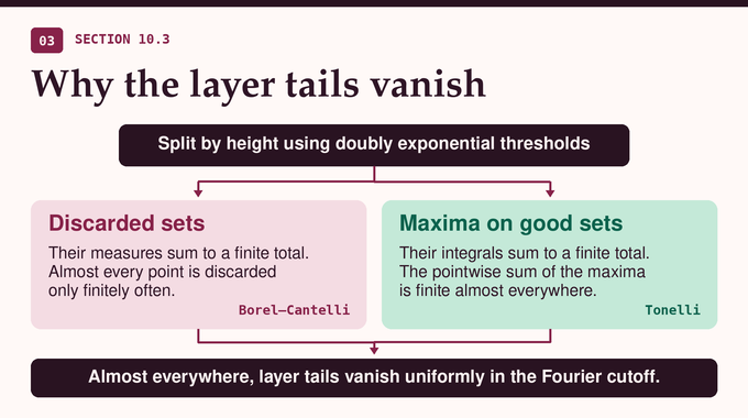
Next, split the unbounded part into layers with heights from up to . After the same four-part split, let be a nonzero layer mass and set , where . The integral controls the sum of the terms. The extra normalization terms are summable too. If , their cost is at most . For smaller masses it is bounded by .
Since , the discarded measures are summable. Borel–Cantelli ensures that almost every point lies in all but finitely many good sets. Tonelli’s theorem and the integral bounds make the layer maxima summable there, after restoring the finitely many remaining bounded layers. Their tail is therefore small uniformly in the cutoff at each such point. Taking the full-sequence limit on finitely many layers and then sending the tail to zero finishes the proof.
Corollary 10.3 uses Stein’s theorem to obtain a weak- bound for in terms of the Luxemburg norm associated with . The Luxemburg norm is the infimum of the positive scaling factors by which one can divide to bring the integral of of its magnitude down to at most one. The inequality controls the measure of each level set of the maximum.
The result establishes a sufficient condition for almost-everywhere Fourier series convergence. Individual exceptional points remain possible, and the theorem gives no uniform error bound. Functions outside the class can still converge. To follow more proofs in harmonic analysis, explore Binary Verse AI’s coverage of ultraflat Littlewood polynomials and the local smoothing conjecture.
When does a Fourier series converge to its original function?
The theorem guarantees that ordinary symmetric Fourier partial sums converge to the original function almost everywhere for every complex-valued function in the L log L class on the circle. The result covers the entire sequence of partial sums.
What is the difference between pointwise, almost-everywhere and uniform Fourier convergence?
Pointwise convergence concerns what happens at an individual point. Almost-everywhere convergence permits an exceptional set of measure zero. Uniform convergence requires one cutoff for each error tolerance that works at every point for all larger cutoffs. OpenAI’s theorem gives almost-everywhere convergence.
What is the L log L condition in Fourier analysis?
Integrate the absolute value of the function times the natural logarithm of two plus that absolute value. This integral must be finite. On the circle this is stronger than plain integrability, yet it allows some functions outside every power-integrability class with exponent greater than one.
How does OpenAI’s proof extend Carleson’s theorem?
Carleson proved almost-everywhere convergence for square-integrable functions, and Hunt extended it to every power-integrability class with exponent greater than one. OpenAI’s proof gives the same convergence guarantee at the L log L endpoint.
Can Fourier series diverge even when the function is integrable?
Yes. Kolmogorov constructed an integrable function whose Fourier series diverges almost everywhere. Plain integrability cannot guarantee convergence.
What is the main mathematical idea behind OpenAI’s L log L proof?
Entropy compression, noisy labels and dyadic path estimates control many modulation frequencies at once. A Hilbert-transform argument transfers that control to ordinary Fourier sums on a good set. Summing across height layers then gives almost-everywhere convergence.
Does the Lean formalization verify every detail of the paper?
The published Lean scope covers the main theorem on full-sequence almost-everywhere convergence. A line-by-line comparison with the manuscript or verification of its other results would require separate checks.