
A spherical wave can arrive quietly, concentrate into a violent peak, and disperse again. The local smoothing conjecture asks how expensive that peak remains when we measure the wave across time. OpenAI’s October 25, 2026 manuscript presents a proof for every Euclidean spatial dimension from two upward, with consequences for Kakeya sets, Fourier restriction, and Fourier summation.
The mechanism is unusually indirect: build a positive conserved tensor, solve an auxiliary quaternionic determinant equation, and transport its energy between two circles. The result retains an arbitrarily small positive Sobolev loss, while its central frequency estimate has logarithmic growth. This is a mathematical bound on concentration, with no demonstrated acceleration of AI training or wave simulation.
Table of Contents
1. What Is the Local Smoothing Conjecture, and Why Do Waves Focus?
Imagine waves traveling inward from a thin spherical shell. Initially their amplitude occupies a large region. Near the meeting time, different directions reinforce one another in a much smaller region. A measurement at that instant can therefore be dramatically larger than the initial measurement.
Sogge’s local smoothing conjecture, proposed in 1991, quantifies the improvement obtained by integrating over a time interval. Large values still count, but their duration counts too. “Smoothing” refers to the derivative cost in an estimate. It does not mean that a reversible wave evolution physically erases fine detail.
The observation is local in time, although the spatial norm in the main theorem covers all Euclidean space. Choosing the interval from one to two fixes the scale of the statement. It is not a claim about uniform control over an infinite observation period.
1.1. Local Smoothing Conjecture: Key Facts
| Feature | Precise Scope |
|---|---|
| Setting | Euclidean space , every integer . |
| Main Estimate | Spacetime control for on ; smooth, rapidly decreasing initial data. |
| Regularity | Order for every ; zero loss at . |
| Evidence | An OpenAI manuscript plus published Lean scope documentation. This article does not independently rebuild the formalization. |
OpenAI’s October 26 release explanation describes the manuscripts as raw research data for academic examination. The distinction between an available proof artifact and community understanding also frames our coverage of AI mathematical proofs.
2. The Euclidean Wave Equation and the Sharp Sobolev Estimate
The standard wave equation is , where adds the spatial second derivatives. The paper studies the half-wave evolution , with . Combining the two half-wave signs recovers the usual wave evolution from its initial displacement and velocity.
An norm measures the size of a function by integrating its absolute value to power , then taking the corresponding root. Larger exponents penalize peaks more heavily. A spacetime norm integrates over position and time. Sobolev regularity additionally charges for high frequencies, through . Define
Theorem 1.1 of Local Smoothing for the Euclidean Wave Equation states
Here is the initial data and the constant may depend on dimension, exponent, and chosen positive , but not on . Fractional derivative orders are allowed. “Every positive epsilon” does not authorize setting epsilon to zero. Only the case explicitly permits that in this theorem.
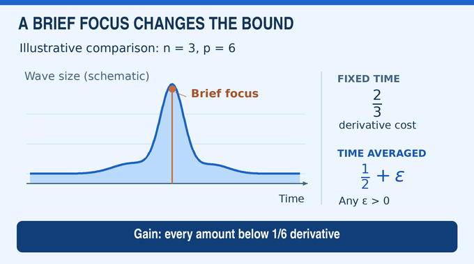
Take three spatial dimensions and exponent six. The threshold is one-half derivative, compared with two-thirds of a derivative at a fixed nonzero time. The difference is one-sixth. The theorem obtains every slightly smaller improvement because of the positive epsilon allowance. This example also shows why smoothing is a comparison between estimates, rather than a claim that every wave becomes visibly smoother as it travels.
3. Why Earlier Proofs Could Not Reach the Critical Exponent in Every Dimension
The difficulty is recombining waves traveling in different directions without overestimating their overlap. Wolff decomposed frequencies into angular sectors and used induction on scales. Bourgain and Demeter’s cone decoupling theorem supplied the near-full smoothing gain for . This still leaves a gap above the conjectured threshold.
In two dimensions, . In three, , while the decoupling threshold is four. Guth, Wang, and Zhang’s sharp cone square-function estimate, published in 2020 after its 2019 submission, settled the planar local smoothing problem.
The new manuscript reviews stronger subsequent three-dimensional results, including full gain up to epsilon for , but distinguishes them from the desired Euclidean critical exponent. At and above , temporal averaging should save every amount below derivatives relative to the fixed-time bound. Below it, the target is arbitrarily small positive regularity. Reaching that junction in every dimension is the central task.
4. The OpenAI Proof’s Central Breakthrough: A Logarithmic Critical Estimate
The proof first isolates one frequency annulus. Let indicate frequency size and , where is a smooth, compactly supported cutoff away from zero. This keeps a band of frequencies comparable to . At , Theorem 1.2 gives
A logarithm grows more slowly than every fixed positive power of frequency. Consequently, this estimate can pay for the small Sobolev allowance in the final theorem. It is much stronger than merely saying that the bound deteriorates by some unspecified power.
For example, in three dimensions the logarithmic exponent is . This describes asymptotic dependence on frequency, not a measured runtime or a numerical accuracy guarantee. Our discrete Fourier transform complexity explainer makes a related distinction between mathematical asymptotics and demonstrated engineering performance. Here the achievement is controlling concentration with the correct derivative threshold.
5. Imaginary Light Rays and Gaussian Localization: Controlling Wave Directions
Complex translation provides the directional filter. For a plane wave with frequency vector , translating spacetime by , with and unit direction , multiplies its amplitude by
This Gaussian favors frequencies aligned with the chosen light ray. For frequencies near , its angular width is of order when is large. These imaginary coordinates are analytical tools, not extra physical dimensions or rays with imaginary speed.
The order of operations matters. The construction adds wave amplitudes first and squares afterward. Squaring each mode separately would destroy cross terms, including the interference responsible for focusing. Gaussian localization therefore has to control direction while retaining the coherent superposition.
Comparable sensitivity to oscillatory cancellation appears in our Littlewood polynomials explainer. Here, however, the Gaussian comes from the wave system’s own flux geometry, giving it a conservation structure that a convenient arbitrary window would lack.
6. Building a Positive Conserved Tensor From the Wave Equation
The wave equation is rewritten as a symmetric first-order system. Its matrix coefficients generate bilinear fluxes with a divergence identity. Applying that structure to the analytically continued wave, together with two auxiliary flows, produces a symmetric positive semidefinite tensor in the enlarged variables.
Positive semidefinite means that every quadratic measurement of the tensor is nonnegative. Conservation means that its real columns have zero divergence. Both properties are needed: positivity prevents cancellation in the energy comparison, while conservation permits integration by parts without uncontrolled interior contributions.
On a suitably narrow, fixed frequency cap, the tensor’s time component still detects the squared size of the original wave through invertible Gaussian multipliers. The proof initially works with finite Fourier sums on a spatial torus, so real spatial integrations have no boundary terms.
There is a subtle obstacle: the unaveraged lifted tensor has a vanishing determinant. The paper therefore smooths and regularizes its time density, obtaining , and uses that scalar as the input to a separate determinant equation. Simply taking the determinant of the original tensor would not deliver the estimate.
The torus here is a periodic box: opposite faces are identified. It makes the algebra finite at a fixed frequency band without restricting the final theorem to periodic waves. Normalizing the nonzero cap data in the energy argument is also temporary. Homogeneity removes that normalization after the comparison.
7. Why a Quaternionic Monge–Ampère Equation Unlocks the Critical Exponent
For each physical time and auxiliary parameter, the remaining coordinates form a spatial fiber. On that fiber the proof solves
Here is an quaternionic Hermitian Hessian, is a large positive parameter, and stays constant along the current. The solution is chosen with positive definite spatial Hessian. Appendix A supplies the required periodic Dirichlet solvability and smooth parameter dependence.
Quaternions extend complex numbers to four real components. Their Hermitian matrices have real eigenvalues, allowing a determinant defined as the product of those eigenvalues. The Hessian collects second derivatives in this algebra. The original wave equation remains linear, even though the auxiliary determinant equation is nonlinear. Its job is to certify an inequality, not to replace the physical evolution.
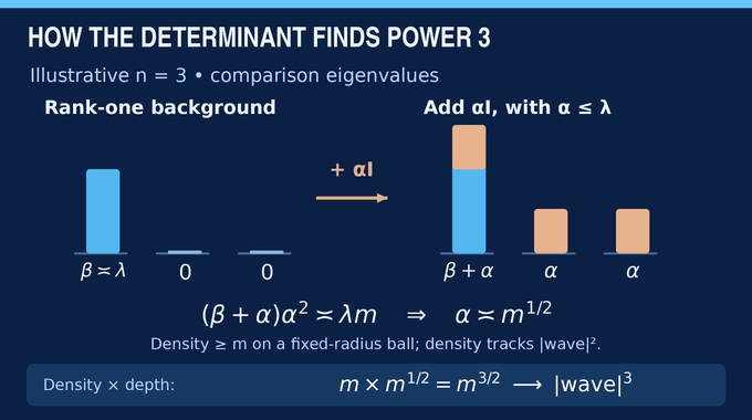
The rank-one background explains the exponent. Its Hessian has one positive eigenvalue comparable to . Adding curvature gives determinant . Thus a density lower bound forces potential depth proportional to , with the geometric radius factor included.
Weighting that depth by density detects . Since the density measures a square of the wave, the resulting wave power is exactly . The quaternionic machinery earns its place by producing the required exponent. This is the decisive link between the auxiliary PDE and the original conjecture.
8. Determinant Energy and the Two-Circle Argument: Where the Logarithms Come From
The first energy candidate integrates potential depth against density. Differentiating it introduces a full determinant without a useful sign. An Aubin–Mabuchi-type correction, integrating determinants along a segment of potentials, cancels that troublesome contribution while preserving comparability with the original positive energy.
Two conservation identities drive the cancellation: one for the current, another for the Hessian cofactor. The fiber geometry makes the cofactor’s normal contribution vanish at the boundary. The remaining positive contribution comes from wave flux through the fiber wall, where Gaussian decay is stronger than the cost of recovering the wave inside.
A cofactor records how a determinant changes when a matrix entry changes. Its divergence identity is therefore the bridge from differentiating the nonlinear determinant to moving derivatives by integration by parts. The boundary calculation matters as much as the interior cancellation: an uncontrolled wall term could undo the whole comparison.
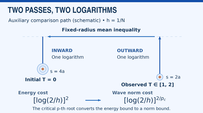
The corrected energy satisfies , where , , and . The comparison moves from a small auxiliary circle outward, connects observation time to initial time at a fixed radius, and returns inward.
Radial harmonic functions in a plane depend on logarithmic radius. Each passage costs a logarithm. The energy therefore loses two logarithms, which become exponent after taking the norm’s root. Section 6 shows both losses can occur for general scalar supersolutions, without proving both are unavoidable for actual waves.
9. From Frequency Caps to All Euclidean Dimensions: Completing the Proof
The cap aperture is fixed independently of frequency. A finite partition of directions therefore covers the annulus without adding another frequency-dependent logarithm. Section 7 transfers the estimate from the torus to Euclidean space using localization and rapidly decaying kernel tails.
Interpolation with the conserved norm and the high-frequency bound supplies the other exponents. A Littlewood–Paley decomposition then separates arbitrary data into dyadic frequency annuli. The extra positive Sobolev allowance makes their weighted contributions summable. This completes Theorem 1.1.
OpenAI’s Lean scope document for local smoothing describes the same dimension range and Sobolev order, including zero loss at two. It also lists formalized consequences for spherical extension, Bochner–Riesz, Kakeya, and Stein’s square function. It should not be read as claiming that every intermediate construction or appendix has been independently audited here.
As our Lean formalization explainer discusses, a formal theorem’s statement and its relationship to the exposition matter alongside machine checking. We have not rebuilt this project or established a completed independent review of the manuscript.
10. Is the Estimate Sharp? Focusing Counterexamples and Endpoint Limitations
“Sharp” requires a qualification. The derivative threshold is forced by examples, but the optimal logarithmic power for unrestricted critical data remains unresolved between the paper’s lower and upper bounds.
10.1. What Sharpness Does and Does Not Mean
| Question | Paper’s Conclusion |
|---|---|
| Derivative Threshold | Radial focusing forces the threshold . |
| Critical Logarithm | Unrestricted annular data require power at least ; the proved upper power is . |
| Zero Regularity | Fails for unrestricted data throughout , even in the weak spacetime norm. |
| Angular Improvement | Positive angular regularity permits the sharp frequency logarithm in the strong critical estimate. |
The focusing example places comparable critical mass at successive dyadic distances from the focus. Counting these scales produces a logarithm. A separate packet construction shows that merely weakening the spacetime norm does not remove every obstruction.
Angular regularity is an additional assumption on the input, not a free improvement. Likewise, Euclidean space is essential to the main theorem’s scope. General curved geometries can impose different thresholds. The paper develops a further symmetric-system extension, but does not establish the identical Euclidean estimate for arbitrary manifolds.
In three dimensions, the critical logarithmic power lies between one-third and two-thirds. Closing that gap requires information beyond the general scalar comparison used here. Also, a theorem in every dimension need not have dimension-independent constants. The estimates allow their constants to depend on the chosen spatial dimension.
11. How the Proof Leads to Kakeya, Fourier Restriction, and Bochner–Riesz
Sections 9–12 convert wave control into other estimates. Near an incoming spherical wave’s focus, rescaling recovers spherical extension. Epsilon removal gives the interior conjectured range for the sphere, and slicing gives the truncated cone. Rescaling small spherical caps also reaches the compact paraboloid.
Random signs on frequency caps then turn extension bounds into tube-overlap estimates. The paper derives Kakeya maximal bounds, hence full Hausdorff dimension for sets containing a unit segment in every direction, for all . Our earlier four-dimensional Kakeya coverage concerns a narrower predecessor. Full dimension does not imply positive Lebesgue measure. Our Falconer distance explainer explores another distinction between dimension and measure.
A projective change yields Nikodym maximal estimates. Time averaging selects thin frequency shells, giving Bochner–Riesz multiplier bounds and Stein square-function estimates at the stated strict orders. The paraboloid argument supplies Schrödinger local smoothing, including the exact spacetime Sobolev order above its critical exponent.
The local smoothing conjecture matters because one precise control on fleeting concentration supports this entire chain. For researchers, the useful next step is understanding the conserved tensor, determinant correction, and endpoint gap. Follow Binary Verse AI for paper-focused explanations that connect the mechanism to exactly what the theorem establishes.
What is Sogge’s local smoothing conjecture?
It predicts sharp spacetime estimates for wave solutions. Averaging over time reduces the Sobolev derivative cost compared with a fixed-time estimate. The manuscript establishes the Euclidean result in every integer spatial dimension , with arbitrarily small positive additional regularity for .
What is the wave equation used in the local smoothing proof?
The standard Euclidean wave equation is . The paper studies its half-wave propagator , with , and bounds its spacetime norm using Sobolev regularity of the initial data.
What is the critical exponent in the local smoothing conjecture?
It is , where is spatial dimension. Thus in two dimensions and in three. Theorem 1.2 establishes a frequency-localized estimate at this exponent with factor .
How does the OpenAI proof differ from earlier local smoothing methods?
Its central mechanism constructs a positive conserved tensor, solves an auxiliary quaternionic Monge–Ampère equation, and compares corrected determinant energies using two auxiliary circles. This differs from earlier approaches organized around cone decoupling, angular square functions, or induction on scales.
Does the local smoothing proof establish the Kakeya conjecture in all dimensions?
The paper derives Kakeya maximal estimates and full Hausdorff dimension of Euclidean Kakeya sets for every . These sets contain a unit line segment in every direction. Full Hausdorff dimension does not assert positive Lebesgue measure. The published Lean scope document lists both the maximal estimate and the dimension consequence.
Does the proof eliminate all epsilon losses and resolve every endpoint?
No. Theorem 1.1 retains an arbitrary positive Sobolev allowance for , while allowing zero loss at . The critical annular estimate has a logarithmic factor. For unrestricted data, the optimal critical logarithmic power remains between and . Lower-bound examples rule out a uniformly lossless estimate in the stated critical and subcritical range.
Has the OpenAI local smoothing proof been formally verified in Lean?
OpenAI reports a Lean formalization. Its scope document covers the Euclidean smoothing theorem with the stated epsilon allowance, plus several consequences including Kakeya, spherical extension, Bochner–Riesz bounds, and Stein’s square function. This article has not rebuilt the project. Published formalization scope should be distinguished from independent review of the full mathematical exposition.