

A perfect triangular grid has a formidable opponent: every disordered arrangement of points in the plane. The opponent can abandon repetition, squeeze distinct points arbitrarily close together, and concentrate enormous crowds in scattered regions. OpenAI’s September 26, 2026 preprint presents a proof that none can beat the grid’s lower energy per particle for an entire class of repulsive interactions.
That is the precise meaning of triangular lattice universal optimality here. The result covers locally finite configurations of centered-disk density one and nonnegative completely monotone potentials of squared distance. Its engine is an atomic interpolation certificate producing sharp Gaussian Fourier minorants. Understanding the achievement requires following three different tasks: certified finite computation, an exact infinite correction, and a global energy comparison.
Table of Contents
1. Triangular Lattice Universal Optimality: The Problem OpenAI Solved
Universal optimality asks one arrangement to win for every interaction in a specified family. Optimizing a single potential could reward a particular distance pattern. Winning across the family requires a common mathematical reason.
The atomic-certificate research paper supplies that reason through Fourier analysis. Its conclusion concerns energy in an infinite configuration, with both the density and energy defined through expanding disks. It is substantially more demanding than comparing repeating grids.
1.1. Key Facts About the Universal Energy Theorem
| Feature | Verified Scope |
|---|---|
| Target | Triangular lattice with fundamental-cell area one. |
| Competitors | Locally finite planar sets with centered-disk density one. |
| Interactions | Smooth, nonnegative completely monotone functions of squared distance. |
| Energy convention | Lower limit of ordered-pair energy per particle. Infinite energies are allowed. |
| Certificate | Sharp Gaussian minorants, two 20×20 finite blocks, and a summable infinite correction. |
| Limits | No classification of minimizers or demonstrated engineering speedup. |
OpenAI included the manuscript in its October mathematics release, describing results produced by an internal frontier model. That attribution establishes provenance, not independent peer review.
2. The Triangular Lattice and Its Energy Minimization Problem
Take two equal-length vectors meeting at sixty degrees, then include every integer combination. The normalization below gives each fundamental parallelogram area one:
For a competitor , let be the closed disk centered at the origin, and let count its points. Density one means . Local finiteness means every bounded region contains finitely many points.
Triangular lattice energy minimization uses the following lower energy per particle:
The function receives squared distance. Every unordered pair is counted twice, once in each direction, so there is no factor of one-half. Only pairs inside the disk enter that disk’s sum. The lower limit accommodates configurations whose averages oscillate instead of converging. These choices determine exactly what the theorem proves.
For a concrete Gaussian interaction, two points separated by one unit contribute a fixed positive amount, while increasing their separation reduces it exponentially. Yet spreading one pair can crowd others. Density fixes the overall space available per point, preventing the trivial strategy of moving every particle indefinitely farther away.
3. Why Earlier Proofs Could Not Cross the Nonperiodic Barrier
Rankin and Cassels, with later corrections and refinements, established triangular minimization for convergent inverse-power lattice sums. Montgomery’s theta theorem established Gaussian minimization among planar lattices of fixed covolume. Neither comparison automatically controls a configuration lacking periods.
Cohn and Elkies developed Fourier bounds for packing. Cohn and Kumar developed energy bounds and the universal-optimality program. Sharp Gaussian auxiliaries later proved the E8 and Leech lattice cases in dimensions eight and twenty-four.
Planar progress also covered particular periodic classes, finite configurations on specified tori, and sufficiently small bounded displacements of the triangular lattice. The last category can include nonperiodic displacements, but it still restricts how far points move.
Here “nonperiodic barrier” describes the unrestricted competitor problem, not an absence of earlier nonperiodic results. Our periodic tiling explainer illustrates why repeating and arbitrary configurations require different arguments.
4. Theorem 1.1: What Universal Optimality Actually Establishes
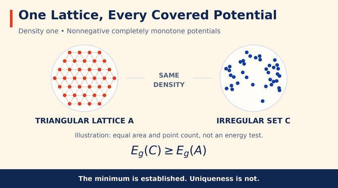
Theorem 1.1 states that every eligible competitor has lower energy at least the triangular lattice’s full neighbor sum:
Completely monotone potentials obey for every integer and . Thus the potential is nonnegative, decreasing, convex, and constrained at every derivative order. Ordinary repulsion alone is insufficient.
Examples include Gaussians and for every . The latter corresponds to distance raised to . In two dimensions its lattice sum converges for and diverges for . The theorem includes the divergent cases as comparisons in the extended nonnegative reals.
Distinct points keep each finite-disk distance positive, even when the potential is singular at zero. No uniform minimum separation is required. Crucially, the theorem identifies a minimum without classifying every arrangement attaining it. As in our quantum circuit lower bounds analysis, the permitted class is part of the result.
The infinite-energy cases need careful interpretation. They do not rank two divergent configurations by a finite energy difference. They say that when the lattice neighbor sum is infinite, every admissible competitor also has infinite lower energy under this convention. No background subtraction or renormalized Coulomb energy is introduced.
5. Theorem 1.2: How Gaussian Fourier Minorants Make the Bound Sharp
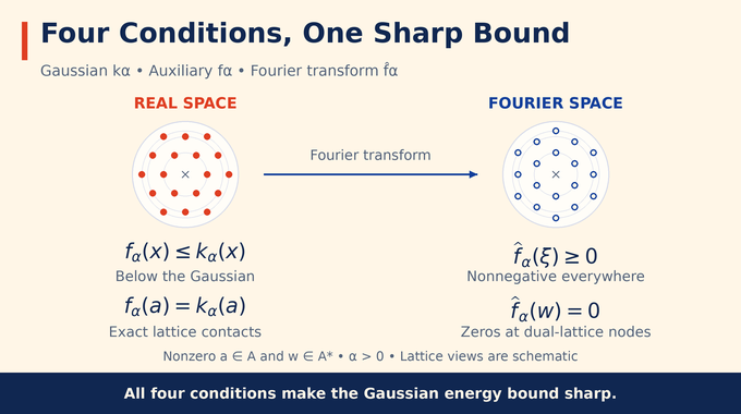
For each , write . Theorem 1.2 constructs a real, radial Schwartz function . “Radial” means it depends only on distance from the origin. Schwartz decay controls the function and every derivative faster than inverse powers.
The last line applies to nonzero lattice points and nonzero dual-lattice points , respectively. The dual lattice consists of frequencies taking integer dot products with every lattice vector.
Each condition has a job. Minorization lowers the competitor’s energy. Fourier positivity provides a universal lower bound. Exact contacts and dual zeros make that bound equal the target energy. A plausible-looking curve satisfying only some conditions proves nothing sharp.
Fourier constraints also drive the Barker sequence argument, although its discrete character calculations solve a different problem.
Think of the auxiliary as an accounting rule. It can sit below the physical interaction, including at distances the target lattice never uses. Its Fourier transform then certifies that every competitor must pay a minimum total bill. Exact lattice contacts ensure the target pays that bill without an overestimate.
6. How Fourier Positivity Overcomes Irregular Point Configurations
For the finite set , form the exponential sum . Fourier inversion turns the sum of auxiliary interactions, including self-interactions, into the integral of over all frequencies.
The decisive lemma says that, after division by , at least unit limiting mass remains in every fixed frequency disk around zero. A smooth disk cutoff and centered density establish this statement. It needs no uniform bound on counts in translated small disks.
Nonnegative Fourier values let the argument discard frequencies outside that disk. Continuity controls those inside. Removing the self-interactions then yields the lower bound .
The density-one triangular lattice has a dual equal to a quarter-turn of itself. Poisson summation, lattice contacts, and dual zeros identify that lower bound with the Gaussian lattice energy. The geometry disappears from the competitor side but remains encoded in the certificate. For another geometric use of Fourier analysis, see our Falconer distance explainer.
7. The Atomic Certificate: Why Modulo-36 Interpolation Works
Set . Triangular-lattice radii then have coordinates . Modulo 36, these occupy fifteen residue classes: 0, 1, 3, 4, 7, 9, 12, 13, 16, 19, 21, 25, 27, 28, and 31.
The OpenAI triangular lattice proof interpolates at every positive integer in these classes, a convenient superset of actual lattice shells. Call the residue set . The following product creates double zeros at every chosen node:
Multiplication by suitable simple-pole and double-pole factors removes the apparent singularities and produces columns prescribing a value and first derivative. Matching both gives tangency, which becomes essential when proving signs between nodes.
The finite periodic columns are trigonometric polynomials before Gaussian damping. Their spectral measures are finite sums of point masses, or atoms. “Atomic” refers to those measures, not physical atoms. Rational tail columns instead have absolutely continuous spectral measures. Their variation bounds are uniform across nodes, allowing summable coefficients to define genuine Schwartz functions.
The extra interpolation nodes are deliberate. Describing every actual triangular shell individually would sacrifice the periodic arithmetic structure. Enlarging the node set gives a tractable sine product, while still including every contact needed for sharpness. The price is proving all those additional constraints consistently.
8. Two 20×20 Systems: Certifying the Finite Gaussian Interpolation
Two input functions are coupled as and . Radiality and Fourier inversion ensure . One side must touch the Gaussian while the other touches zero.
Ten positive nodes supply twenty value-and-derivative coordinates on each side. Adding and subtracting the two sides separates the forty coupled coordinates into two 20×20 systems. Data at zero and designated constant terms are fixed separately.
For , one containing polytope encloses the parameter-dependent Gaussian data. Outward-rational interval arithmetic certifies inverses and coefficient bounds. Bernstein polynomial coefficients certify inequalities throughout the polytope, rather than at sampled parameter values.
8.1. What Each Certificate Layer Establishes
| Layer | Contribution | Remaining Obligation |
|---|---|---|
| Finite arithmetic | Certified 20×20 inverses and polynomial margins. | Restore all omitted interpolation data. |
| Infinite correction | Exact values and slopes at every positive node. | Prove inequalities between the nodes. |
| Global analysis | Signs at every radius and the density-based energy bound. | Transfer Gaussian inequalities to the full potential family. |
This smaller finite construction differs from the paper’s modulo-12 companion, whose blocks use 168 positive-node coordinates each. Smaller matrices do not enlarge the competitor class or remove the analytic work.
Interval arithmetic encloses exact quantities between certified lower and upper endpoints. Rounding outward prevents numerical error from manufacturing a positive margin. Bernstein bounds address a separate issue: a polynomial is a weighted combination of its Bernstein coefficients on an interval. Controlling all coefficients controls the whole interval, including unsampled points.
9. The Infinite Correction: From Finite Data to Exact Interpolation
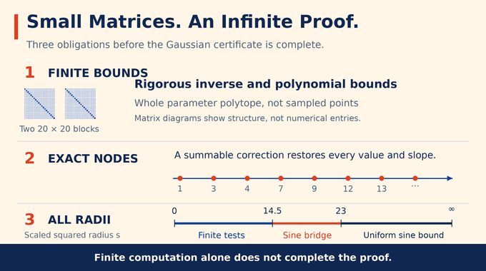
A finite interpolant leaves residual errors. It omits some Gaussian target data and fails to control infinitely many later nodes. Periodic columns also repeat their contributions in later residue classes. Stronger damping makes those repetitions small, not zero.
The proof places tail coefficients in , meaning their absolute values have a finite sum. Schur elimination removes the finite variables, leaving an operator equation on the entire tail space. A norm bound strictly below one permits inversion by a convergent Neumann series.
Proposition 5.1 bounds each tail coefficient norm below and each finite-coordinate correction below . These are coefficient-space bounds, not automatically pointwise function errors. Curvature estimates subsequently convert them into the control the sign proof needs.
Uniqueness here concerns coefficient lists with prescribed fixed columns. It does not assert uniqueness among all radial Schwartz interpolants. The need for bounds surviving an infinite limit also appears in our Bose–Einstein condensation explainer.
For a developer, this is the difference between solving a truncated linear system and proving that an infinite system has a solution nearby. The finite answer becomes useful only after a stability estimate limits the omitted interactions. Tiny residuals alone cannot establish that stability.
10. Proving the Fourier Inequalities Between Every Interpolation Node
Exact values at infinitely many nodes still leave infinitely many gaps. A function can touch the right values and misbehave between them. Our Littlewood polynomial explainer examines a related demand for control at every angle.
Near a node, the proof subtracts the known value and linear term, then divides by squared displacement. The resulting divided remainder is controlled by second derivatives. Degree-twenty Taylor polynomials, Bernstein bounds, and correction estimates settle whole half-cells, not a plotting mesh.
The first right half-cell needs special treatment. Its Gaussian comparison is rational in the parameter. Clearing a positive quadratic denominator creates a cubic inequality, certified through four Bernstein coefficients. Applying the generic estimate there would leave a gap.
Finite tests cover . Beyond that, fixed terms with opposite signs multiplying dominate the remaining curvature. A stronger sine-product bound bridges , followed by a uniform periodic bound. The interpolation functions themselves need not be periodic. Positive normalization finally produces the required Gaussian minorant.
This last step is easy to underestimate. A dense numerical plot cannot exclude a narrow sign violation, particularly near a tangency where the available margin vanishes quadratically. Dividing out the known contact separates that unavoidable vanishing from the positive remainder that must actually be certified.
11. From Gaussian Energies to Universal Optimality: Completing the OpenAI Proof
Reciprocal-parameter duality extends the construction from to every positive parameter. In two dimensions the Gaussian transform is . Taking gives the complementary minorant, preserving the required inequalities and contacts.
The Bernstein–Widder representation then expresses every eligible potential as a positive mixture:
Each positive mixing parameter gives a Gaussian inequality. Fatou’s lemma passes the lower limit through the nonnegative mixture, and Tonelli’s theorem exchanges integrals and lattice sums. The argument includes infinite representing mass and an atom at zero, which contributes a constant interaction.
It mixes energy inequalities, not auxiliary functions. Consequently, it does not automatically construct the separate sharp auxiliary for every mixed potential requested by the stronger Cohn–Kumar formulation.
The published Lean scope documentation reports formalization of the universal energy theorem and sharp Gaussian minorants, including the atomic construction in its stated parameter range. We have not independently rebuilt that code. Formal checking and mathematical peer review answer different questions, a distinction also relevant to our Courtade–Kumar coverage.
For developers, the reusable lesson is how finite certified computation supports an infinite analytic theorem. As with mean-payoff games complexity guarantees and trace reconstruction lower bounds, this is not a demonstrated application benchmark. Triangular lattice universal optimality supplies a rigorous energy target under precise assumptions. Follow Binary Verse AI for research explainers that connect each proof’s mechanism to exactly what it establishes.
What does triangular lattice universal optimality mean?
It means the density-one triangular lattice minimizes the lower energy per particle for every nonnegative completely monotone potential of squared distance, among locally finite planar configurations with the same centered-disk density. It is an energy-minimization theorem, rather than merely a circle-packing result.
Does the OpenAI proof apply to nonperiodic and irregular point arrangements?
Yes. Theorem 1.1 includes nonperiodic arrangements, arbitrarily close distinct points, and highly irregular local concentrations, provided local finiteness and centered-disk density one hold. No bounded-displacement condition or uniform minimum separation is required.
What kinds of repulsive interactions are covered?
The theorem covers smooth, nonnegative completely monotone functions of squared distance. These include Gaussian interactions and inverse powers for . Infinite energies are allowed. Not every physically repulsive potential satisfies complete monotonicity.
Why are Gaussian Fourier minorants central to the proof?
They provide energy lower bounds through Fourier positivity. Exact agreement with the Gaussian at nonzero triangular-lattice points, together with Fourier zeros at nonzero dual-lattice points, makes the lower bound sharp for the target lattice.
How does the atomic certificate prove infinitely many conditions?
The proof first certifies finite interpolation bounds using two 20×20 systems and rigorous arithmetic. It then constructs an absolutely summable infinite correction and proves the required signs at every radius. Finite computation alone does not complete the proof.
Does the proof show that the triangular lattice is the unique optimal arrangement?
No. Theorem 1.1 identifies the minimum energy without classifying all arrangements attaining equality. It also does not, by itself, construct the separate sharp auxiliary for every mixed potential requested by the stronger Cohn–Kumar formulation.
Is the OpenAI proof computer-assisted, and has it been formally verified?
Yes. The manuscript combines rigorous finite arithmetic with analytic arguments controlling infinitely many interpolation conditions. OpenAI’s Lean documentation reports formalizations of the universal energy theorem and sharp Gaussian minorants, including the explicit atomic construction in its stated parameter range. This article has not independently rebuilt the Lean project. Formal verification is distinct from independent mathematical peer review.