

Delete one bit and every later position can become ambiguous. Delete bits independently across repeated copies, and even unlimited computation may need more observations than any fixed polynomial can supply. That is the central result of OpenAI’s September 24, 2026 paper, Quantitative Lower Bounds for Trace Reconstruction.
For every fixed deletion probability strictly between zero and one, exact worst-case trace reconstruction requires independent traces. The proof rules out a universally sufficient polynomial sample count. Its mechanism hides deliberately arranged differences inside uncertainty about their locations, then repeats that concealment across scales. This is an information limit for a precise mathematical model, without a demonstrated sequencing benchmark or recovery-system speedup.
Table of Contents
1. What Is Trace Reconstruction, and Why Do Deleted Bits Make Recovery Difficult?
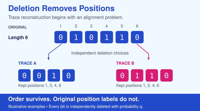
An unknown binary string has length . The deletion channel independently removes each bit with known probability , retaining it with probability . A complete trace contains every surviving bit in its original order, together with the resulting length. Original positions are absent. Different traces use independent deletion decisions on the same fixed string.
For example, start with 010110. Retaining positions 1, 3, 4 and 6 gives 0010. Retaining positions 1, 2, 4 and 6 instead gives 0110. These are illustrative deletion patterns, not equally likely outcomes asserted for every channel. Missing position labels make alignment part of inference.
1.1. Trace Reconstruction: Key Facts
| Research Detail | Precise Scope |
|---|---|
| Input | One deterministic, arbitrary length- binary string. |
| Observation | Independent complete traces, with lengths and surviving symbols visible. |
| Channel | Known , fixed across samples within an instance. |
| Guarantee Ruled Out | A polynomial sample budget sufficient for every input at fixed positive success. |
| Computing Resources | Unrestricted computation, including randomized estimators. |
| Evidence | A written preprint, with separately documented Lean scope; no practical benchmark. |
The biological motivation concerns sequence alignment under missing symbols. However, this theorem studies binary deletion traces, rather than directly measuring four-letter DNA recovery. It also differs from shortest common superstring, where fragments must occur contiguously in an assembled string.
2. The Original Problem: Can Polynomially Many Traces Recover Every Binary String?
Worst-case reconstruction demands one procedure that succeeds on every possible input, including adversarially chosen strings. The paper writes for the smallest fixed trace budget achieving success at least on every length- input. The estimator knows the length and channel. Conventionally, success is .
The old question was whether some constant exponent could always suffice. Proving that particular strings require many observations would settle it negatively only if the requirement eventually exceeded every fixed power of length.
Sample complexity counts observations. Computational complexity counts the work needed to process them. Infinite processing power cannot recover distinctions absent from the data. Our quantum query complexity explainer similarly separates information access from intervening computation. Here the observations are complete traces, and no restrictions on the chosen statistics rescue a polynomial guarantee.
3. The Previous Barrier: Why Earlier Lower Bounds Remained Polynomial
Earlier constructions hid a small defect inside a long repetitive background. Random deletions blurred its apparent position. Holden and Lyons obtained a requirement of order . Chase’s lower-bound paper strengthened the worst-case rate to . These comparisons fix the channel and use reconstruction success greater than one-half.
Those were substantial obstructions, but still compatible with a higher-degree polynomial working universally. A lower bound near the three-halves power cannot exclude a quadratic or hundredth-power sample budget.
Stronger impossibility statements for restricted statistics also existed. Yet excluding coordinate means or local statistical queries does not exclude algorithms exploiting the entire trace. This model distinction matters just as it does in quantum circuit lower bounds: the resources permitted by the theorem determine what its conclusion excludes.
4. What the OpenAI Proof Establishes: A Superpolynomial Sample Lower Bound
Theorem 1.1 fixes and a constant . Along any sequence with length tending to infinity and , it gives, eventually:
All logarithms are natural. The deletion probability may vary between instances, but stays fixed throughout each instance’s construction and observations. At any fixed positive deletion probability below one, the exponent grows like log log length. Hence the bound exceeds every fixed polynomial eventually. It supplies no numerical threshold for ordinary data sizes.
The quantifiers are the breakthrough. Choose any proposed polynomial budget, with its exponent fixed in advance. At sufficiently large lengths, some inputs defeat that budget. The theorem does not identify one finite string that defeats every sample count, nor claim that randomly chosen inputs typically resemble its carefully constructed hard examples.
Theorem 1.2 isolates the statistical reason. For one-trace laws and , total variation measures their distinguishability:
The sum runs over finite binary outputs. At each fixed channel, the minimum distance between distinct length- strings becomes smaller than for every fixed , asymptotically. These distributions need not be identical. Their differences simply become too faint for polynomially many samples to reveal reliably. Unlike the bit-flip setting in our Courtade–Kumar explainer, deletions hide alignment as well as information.
5. The Initial Construction: Alternating Strings With Carefully Shifted Defects
The seed starts with ordinary blocks and defect blocks . Each period contains one defect among alternating blocks. Moving that defect by one block slot changes the word while preserving its length. Across selected periods, the two candidate words move defects in opposite directions according to a signed pattern.
The proof introduces an auxiliary observation retaining ordered marks but hiding original slot labels. Joining those marks produces an ordinary deletion trace. This gives the analysis extra information while preserving a route back to the actual channel.
Its likelihood score, , compares auxiliary laws: zero indicates local agreement, while deviations record statistical evidence. Here the derivative denotes a likelihood ratio. The seed bounds moments of this score and establishes overlap between traces of consecutive repeated powers. Both properties are needed later. A hard pair alone would not provide everything required for recursive concealment.
6. Hidden Offsets: How the Proof Makes Different Strings Look Alike
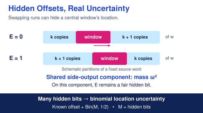
Suppose traces of and share probability mass . Put these runs on opposite sides of a central segment. A fair orientation bit decides which side receives the longer run. Both orientations have the same total length.
The paired laws share a product component of mass . On that component, even reporting both side outputs does not reveal the orientation. Outside it, the auxiliary observation may reveal the bit. Averaging over the flags restores the correct side-trace laws.
With many independent pairs, unrevealed fair bits accumulate. Conditional on the report, their contribution to the central segment’s location is a known offset plus , where counts hidden orientations. Thus an adversary cannot precisely place the statistical discrepancy.
Crucially, the original word remains deterministic. Randomness chooses a partition used to generate an observation, rather than changing the source string. Confusing these would substitute a different reconstruction problem for the one being proved hard.
For deletion probabilities above one-half, the construction first works at one-half and then deletes additional surviving bits to obtain the requested channel. Common postprocessing can only reduce distinguishability. For smaller probabilities it works directly at the requested rate, which remains unchanged through all intermediate scales.
7. Prouhet–Thue–Morse Cancellation: Why Statistical Differences Disappear
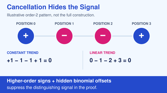
Uncertain position becomes especially effective when neighboring discrepancies have coordinated signs. For cancellation order , the Prouhet–Thue–Morse signs satisfy:
Every factor vanishes at , giving a zero of order . A small example is the sign pattern plus, minus, minus, plus. Its total is zero, and its position-weighted total is also zero: zero minus one minus two plus three. It cancels constant and linear trends.
The proof uses much higher orders. Averaging a signed pattern over a broad binomial location distribution convolves the two sequences. Finite-difference cancellation suppresses the resulting signal. Fourier estimates quantify that suppression while tracking dependence on channel and cancellation order.
The signed-sequence algebra recalls Barker sequence cancellation, although the required property here is a high-order polynomial zero, rather than small aperiodic autocorrelations. Cancellation alone still does not control all interactions. That is the next obstacle.
8. The Forced Binary Subtree: How Small Differences Become Even Harder to Detect
Nested segments form a tree. Expanding the conditional likelihood difference produces terms indexed by selected leaves, each carrying an old likelihood score. The complementary words have opposite root signs, so subtracting their expressions cancels every even root term.
An odd term with only one active child at an odd vertex contains a singleton signed factor. The hidden local offset smooths that factor through the previous cancellation estimate. These contributions become negligible.
For any remaining odd root term, every selected odd internal vertex must have at least two active children. Choosing two recursively forces a complete binary subtree with leaves at depth . At , for example, that forces eight old-score factors.
Multiplying many small scores helps, but does not supply the entire improvement. Siblings also share a global displacement while retaining independent local displacements. A joint location bound preserves that dependence and supplies additional decay. Treating sibling positions as independently scattered would lose an essential part of the argument. Recursive construction matters here, as in the quadratic sensitivity counterexample, because each stage must preserve the properties needed by the next.
9. Multiscale Amplification: Turning a Polynomial Obstruction Into a Superpolynomial One
The induction tracks three quantities: likelihood-score moments, approximation error when projecting to genuine traces, and overlap between consecutive repeated powers. If any one fails, the next hiding step may be unavailable or its apparent statistical gain may be illusory.
Write the squared score strength at target scale as . One depth- amplification block updates its exponent by . The small subtraction reserves margins for other losses. This is the paper’s quantitative recurrence, rather than a measured performance improvement.
The schedule has two phases. Initial blocks strengthen the seed sufficiently to justify later, deeper blocks. Repeated gains across a number of blocks growing like log log length then produce an exponent of that order.
Hellinger distance connects the machinery to testing. It contracts under common postprocessing, and its squared value for independent products is bounded by the sum of the individual squared distances. Likelihood moments control it while also keeping exceptional events small enough across all scales. Probability estimates must survive repetition, a concern also central to sampling guarantees for counting perfect matchings.
9.1. What Each Induction Estimate Protects
| Estimate | Role in the Next Stage |
|---|---|
| Score Moments | Keep likelihood differences small and control higher-degree terms in their expansion. |
| Consecutive-Power Overlap | Preserve common probability mass so paired runs can hide fresh orientation bits. |
| Projection Error | Bound the discrepancy between the auxiliary observation after postprocessing and the genuine trace law. |
The construction therefore cannot spend its entire gain on making the current pair close. It must leave enough overlap and enough error margin to build another pair. This is why the initial strengthening phase and the constants in the recurrence belong to the mechanism, rather than being decorative technical bookkeeping.
10. Completing the Proof: From Auxiliary Observations to Genuine Deletion Traces
Auxiliary observations cannot be substituted silently for the real experiment. The proof explicitly maps them back, charging errors for failed layouts, inherited approximations and conditioning. Clipping restricts to typical metadata and a region where the reference density satisfies , making likelihood ratios manageable. The excluded mass remains within the error budget.
The constructed pair may be shorter than requested. Appending the same tail produces distinct words of exactly the target length. Generating an independent tail trace and concatenating it cannot increase distinguishability.
With and now denoting the genuine trace laws, final score exponent and per-law projection error , the product bound has the form:
Here is the trace budget. Keeping this distance small limits the success of every two-hypothesis test. To cover any fixed positive reconstruction success, even below one-half, the proof combines independent hard gadgets. Their separated observations provide extra information, yet posterior factorization bounds joint success by for gadgets. Choosing a fixed sufficiently large completes the extension.
11. What the Proof Resolves, and What Remains Open
The result resolves the polynomial-sample question negatively for exact worst-case binary reconstruction at fixed deletion probability. It does not say every input is difficult. The manuscript cites polynomial algorithms for sufficiently separated strings and for deletion rates with fixed , outside its varying-channel regime.
Nor does it determine the optimal rate. Burudgunte, Valiant and Wang’s quasipolynomial sample upper bound leaves a gap above the new lower bound. Their paper explicitly separates sample complexity from general reconstruction runtime. This manuscript also cites a companion time-bound result under fixed rational retention probabilities. Neither citation turns this lower-bound paper into a practical decoder.
Superpolynomial also does not mean exponential in the string length. The new lower bound grows faster than every fixed power, while remaining below familiar exponential scales. Confusing those categories would overstate the result substantially.
Recovery is still possible in principle: a trace occasionally suffers no deletions, and its known full length identifies it as the original word. Repeating observations can make that event highly likely, though waiting for it is inefficient. The theorem asks how many samples are necessary for a uniform guarantee, not whether any successful observation can ever occur.
OpenAI’s mathematics release announcement attributes the collection to an internal frontier model. The result-specific Lean scope note describes the quantitative and superpolynomial conclusions. The comparator configuration points to a separate solution module containing proof code. Comparator placeholders are statement targets, not that implementation. This review did not independently compile the development. Written arguments, formal verification and practical validation answer different questions.
For developers, the useful lesson is to state input promises, channel assumptions and exactness requirements before judging recovery performance. A successful benchmark on ordinary inputs does not establish a worst-case guarantee. Trace reconstruction now has a sharper mathematical limit: additional computation cannot replace missing observational evidence. Follow Binary Verse AI for research explainers that trace such conclusions back through the arguments that support them.
12. Frequently Asked Questions
What is the trace reconstruction problem?
Trace reconstruction asks how to recover an unknown original string from independently generated copies in which each symbol is deleted with a known probability. Surviving symbols retain their relative order, but their original positions are unknown.
What did the OpenAI trace reconstruction proof establish?
For every fixed deletion probability strictly between zero and one, the paper proves that exact worst-case binary reconstruction requires traces at any fixed positive success probability, even with unrestricted computation. This rules out a universally sufficient polynomial sample bound.
Why were previous trace reconstruction lower bounds insufficient?
Earlier bounds were polynomial, including Chase’s lower bound at a fixed channel and success greater than one-half. They could not rule out a higher-degree polynomial number of traces always sufficing.
How does the OpenAI proof make different binary strings statistically indistinguishable?
It combines shifted defects, hidden binomial offsets, Prouhet–Thue–Morse cancellation and repeated multiscale amplification. These constructions make the complete trace distributions extraordinarily close, rather than necessarily identical.
Can more computing power overcome the trace reconstruction lower bound?
No. The theorem permits unrestricted computation. For its worst-case inputs and sample budgets, the obstacle is insufficient statistical information in the observed traces, rather than the time required to process them.
Does the proof mean that reconstructing deleted information is impossible?
No. It rules out polynomial sample complexity for exact worst-case reconstruction at any fixed positive deletion probability below one. It does not rule out recovery with more traces or polynomial reconstruction under certain restricted input or channel conditions.