
Adding four bits modulo two is easy. Proving that a powerful family of shallow quantum circuits cannot reliably do the same job took a much subtler argument. OpenAI’s September 24, 2026 paper establishes quantum circuit lower bounds excluding parity from QAC⁰, even with polynomially many workspace qubits, arbitrary discarded outputs, and any fixed positive worst-case advantage over guessing.
The result resolves Moore’s parity conjecture in the measured-output model. Its engine is product-projection localization, a theorem controlling how shallow circuits connect product conditions to states with many mismatches. This is a mathematical impossibility result for a specified circuit model. Understanding the proof means understanding exactly which resources that model permits.
Table of Contents
1. Why Is Parity So Difficult for Shallow Quantum Circuits?
Parity reports whether a bit string contains an odd number of ones. XOR, written , adds bits modulo two:
For 1011, three ones produce parity one. For 1010, two ones produce zero. Flipping any single input flips the answer, so parity depends sensitively on every position.
That does not make parity universally difficult. A sequential circuit can accumulate XORs, and a tree can combine partial answers. The question is whether quantum interference and very large gates can compress this global dependence into a fixed number of layers.
1.1. Quantum Circuit Lower Bounds: Key Facts
| Gate Set | Arbitrary one-qubit unitaries and unbounded-arity Toffoli gates; disjoint supports per layer. |
|---|---|
| Resources | Fixed depth ; input qubits; at most total qubits for fixed . |
| Input and Output | Ancillas start at zero. One output is measured; all final garbage is unrestricted. |
| Excluded Guarantee | Success at least on every input for fixed , at sufficiently large input lengths. |
| Evidence | Theorems in a research preprint, with accompanying Lean formalization of parity and localization; no hardware benchmark. |
Here depth measures sequential layers of gates acting on disjoint sets of qubits. Unlike quantum query complexity, which counts accesses to input information, this problem restricts how the computation itself is organized.
2. Moore’s Parity Conjecture: The Problem That Remained Open
Classical AC⁰ permits constant-depth, polynomial-size circuits with unbounded-input AND and OR gates, plus NOT. Established classical results exclude parity. Quantum QAC⁰ instead permits arbitrary one-qubit unitaries and unbounded-arity Toffoli gates, subject to disjoint gate supports within each parallel layer.
Moore connected coherent parity with quantum fanout in 1999. His original formulation required ancillary qubits, the temporary workspace, to return to zero. Computing one measured answer while leaving arbitrary garbage is more permissive than implementing a clean reversible transformation.
Earlier quantum bounds restricted ancillas, depth, approximation requirements, or output cleanliness. For example, Fang and colleagues obtained a logarithmic depth lower bound depending on the number of ancillas for exact clean parity. Later spectral approaches extended bounded-error exclusions to larger but restricted ancillary registers.
The remaining challenge was simultaneous freedom: every fixed depth, every fixed polynomial qubit budget, bounded error, and unrestricted final garbage. Classical wire reuse also prevents directly transplanting an AC⁰ proof into this quantum model.
3. The Exact Quantum Circuit Lower Bound OpenAI Proved
Theorem 1 of the original product-projection localization paper fixes a nonnegative integer depth , a real exponent , and an advantage . For sufficiently large input length , no permitted circuit with depth at most and total qubit count succeeds with probability at least on every input.
The input is a computational-basis string, with all additional qubits initialized to zero. One designated output qubit is measured in the computational basis. The input need not survive, and remaining registers may be discarded without cleaning them.
Choosing gives the familiar two-thirds success requirement. The theorem says every sufficiently large circuit meeting the resource limits has some input below the chosen success threshold.
The order of quantifiers matters. Depth, polynomial exponent, and advantage are fixed before input length grows. It supplies no universal small-input cutoff and no hardware timing estimate.
The circuits may depend on input length without being efficiently generated, so the exclusion also covers nonuniform circuit families. They cannot depend on the particular input string. Polynomially many total qubits also bound the gate count, because each disjoint layer contains at most one nonempty gate per qubit.
4. Why Unbounded Toffoli Gates Defeat Ordinary Light-Cone Arguments
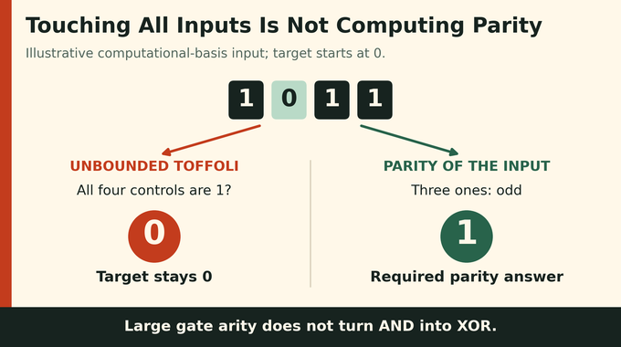
A Toffoli gate flips its target when all its control bits are one. Here the number of controls is unrestricted. One gate can therefore touch every input, making a simple backward light-cone argument ineffective: the output’s dependencies can immediately reach the whole register.
But touching every input does not calculate XOR. With a zero target and controls 1011, that Toffoli leaves the target zero although parity is one. Its trigger tests a conjunction, not the oddness of the total count.
Primitive unbounded fanout is different: one control flips arbitrarily many target bits. Hadamard conjugation interchanges coherent fanout and coherent parity transformations. The paper explicitly excludes fanout as a primitive.
Nor may many simultaneous CNOTs share one control under the disjoint-support rule. Treating that pattern as a single layer would silently change quantum circuit depth. The gate restrictions are therefore substantive, not bookkeeping conventions.
5. Turning Toffoli Gates Into Product-State Reflections
The proof enlarges the gate model to reflections about product projections. A projection selects a subspace. A product projection fixes specified one-qubit vectors on a chosen subset and leaves every other qubit unrestricted.
Let project onto all controls being one. Since the Pauli bit flip satisfies , the controlled gate becomes:
Here is the identity, denotes a tensor product, and . The reflection reverses the sign of the selected component while preserving its orthogonal complement.
The enlarged model alternates arbitrary one-qubit layers with disjoint product-reflection layers. Its depth counts reflection layers, bounded by the original physical depth. Proving localization for this larger class covers the stated Toffoli circuits.
This rewrite also exposes the algebra needed for induction. Reversing the circuit preserves reflection depth, a property used when the proof later invokes , the inverse unitary.
6. Product-Projection Localization: The New Mathematical Principle
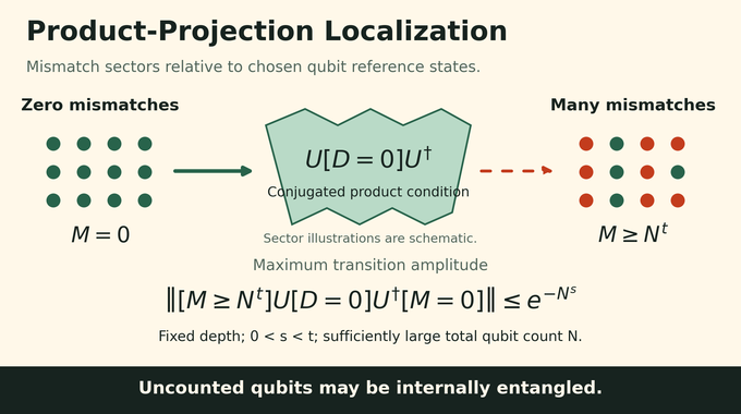
Choose reference vectors on a qubit subset . Define a mismatch count:
Each summand detects the component orthogonal to its reference vector. The summands commute, so their joint eigenvalues count mismatches. Brackets denote spectral projections: selects no mismatches, while selects at least .
For another such count , the condition is a product projection. Theorem 2 states:
For every fixed reflection depth and fixed , this holds for sufficiently large , uniformly over circuits, counted subsets, and reference vectors. The double bars mean operator norm, the maximum output length over unit-length inputs.
Read operators from right to left: start with no mismatches, apply the conjugated product projection, and inspect the high-mismatch component. Its amplitude is suppressed. Uncounted qubits may contain arbitrary internal entanglement.
This is localization in mismatch sectors, rather than physical position or the disordered-lattice phenomenon discussed in Anderson localization.
7. The First Induction: Reducing Circuit Depth
At reflection depth zero, the circuit contains only one-qubit operations. Conjugating a product projection preserves its product structure. Creating mismatches then competes with the amplitude lost when imposing those projections.
For intuition, projecting onto loses half the squared norm. Repeating across many qubits can generate substantial conditional mismatch probability, but the unnormalized surviving amplitude becomes tiny. Renormalizing would erase the penalty that makes the bound work.
For positive depth, first consider a projection supported on qubits. In one disjoint reflection layer, at most gates intersect that support. All other reflections commute past the projection and cancel.
Expanding the remaining reflections on both sides has total absolute coefficient cost at most . Each term becomes three ordered projections conjugated by a shallower circuit. Intermediate mismatch cutoffs ensure that reaching the final high-count sector requires a suppressed transition between factors.
The preceding-depth estimate also extends from zero mismatches to low-count sectors by summing over mismatch patterns. Strict gaps between chosen exponents absorb both this counting cost and the reflection expansion.
8. Why Chebyshev Polynomials Enter a Quantum Circuit Proof
Small support is not enough: the product condition might constrain almost every qubit. The proof therefore approximates its zero-count projector by a polynomial .
One factor has exact roots at the first several positive integers, eliminating those mismatch counts outright. A normalized Chebyshev factor suppresses the remaining integer counts across a chosen interval while retaining . Chebyshev polynomials stay bounded on their standard interval and grow rapidly outside it, enabling this separation.
Approximation error alone is insufficient. Expanding a count’s th power produces up to terms. The paper therefore tracks:
Each monomial becomes a product projection supported on at most qubits. Controlling degree and weighted coefficient norm lets the small-support theorem pay for their entire expansion.
More precisely, Lemma 3 chooses fixed and . It obtains degree at most , weighted coefficient norm at most , and error at most at positive integers through . These inequalities balance approximation strength against expansion cost, leaving room between the exponents used by localization.
Crucially, the polynomial only needs to approximate the projector over a low-count interval. Its behavior at higher counts is handled by the second induction. Demanding a uniform approximation everywhere would miss the proof’s main economy.
9. The Finite-Scale Induction That Completes Localization
Write , , and . The proof squares the transition norm:
Replacing only the first by its polynomial approximation places the error against . This order matters because these operators need not commute.
The low-count error is controlled by the polynomial. Conjugating the remaining high-count term by produces another localization problem, with the two mismatch counts exchanged. It has the same circuit depth but a larger mismatch threshold.
That sounds circular until the thresholds are organized. To establish the exponent pair , one uses an already established pair , where . A finite chain pushes the threshold exponent beyond one, where no count on qubits can reach .
The proof starts at that trivial endpoint and works backward. Its outer induction reduces depth, while its inner induction descends through finitely many scales. Both preserve uniform thresholds over all circuits and reference vectors.
10. From Localization to Parity: The Final Fourier Contradiction
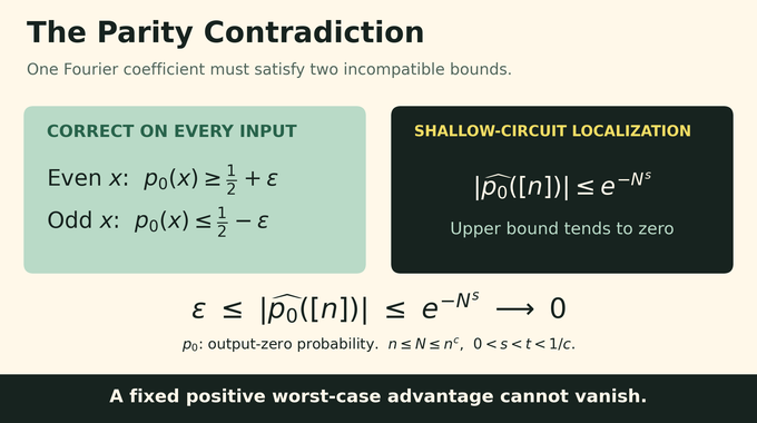
Let be the circuit and the output-zero projection. Define , so is the probability of measuring zero. The trailing zero represents every initially zero ancilla.
The full-parity Fourier coefficient averages this probability with positive signs for even strings and negative signs for odd strings:
Here means all input positions, and counts ones. This Boolean Fourier analysis concerns correlations with parity patterns. It differs from computing the numerical transform in our discrete Fourier transform complexity explainer.
The paper identifies this coefficient with the average of matrix entries of between complementary Hadamard product states. Each coordinate is or ; complementary states exchange every choice and therefore differ on all inputs.
Expanding those states in the computational basis introduces Boolean characters. Averaging over their sign choices cancels every off-diagonal contribution by character orthogonality. The surviving diagonal terms acquire exactly the alternating parity signs in the coefficient above.
Choose . Since , eventually , so localization bounds every complementary entry. Meanwhile, worst-case success forces even inputs above and odd inputs below . Equal class sizes give:
A fixed positive advantage cannot approach zero. That contradiction proves the QAC⁰ parity lower bound without restricting the final garbage.
11. Beyond Parity: Majority, Fourier Concentration and Dicke States
Localization also constrains other global correlations. Section 7 derives Fourier concentration directly and combines structural estimates with earlier reductions and state constructions for additional consequences.
11.1. Consequences and Their Required Qualifications
| Strict Majority | No fixed-depth, polynomial-qubit family achieves worst-case advantage for any fixed at all sufficiently large lengths. |
|---|---|
| Fourier Concentration | For the expected measured output sign, the total squared Fourier weight on subsets of size at least is at most , for every fixed and , eventually. |
| Dicke-State Preparation | For zero-initialized, fixed-depth, polynomial-qubit preparation, trace distance from the weight- Dicke state exceeds when , for fixed , eventually. |
The state-preparation obstruction additionally excludes inverse-polynomial measurement probabilities for both a string and its bitwise complement. Discarding other registers remains allowed.
For majority on uniformly random inputs, Corollary 11 excludes average success at least for every fixed . It does not establish a constant average-case gap. Worst-case advantage and near-perfect average accuracy are different guarantees.
Dicke states are equal superpositions of all strings with a fixed number of ones. The stated trace-distance restriction matters: excluding highly accurate preparation in a specified weight range does not prohibit every approximation or every weight. Likewise, Fourier concentration controls the absolute squared tail of the expected output sign, not a normalized percentage of that function’s Fourier weight.
12. What the OpenAI Proof Establishes and What It Does Not
OpenAI included the preprint in its October mathematics release. As checked on October 22, the Lean formalization scope notes list both general positive-advantage parity and product-projection localization. They explicitly distinguish these from regular-trajectory propagation and pruning, which are not separate formalized statements there. That distinction illustrates the importance of checking formalization scope. This article does not report an independent Lean build or peer-review certification.
The theorem excludes intermediate measurement, postselection, and primitive unbounded fanout. It assumes polynomial total qubits and fixed depth. It supplies neither a quantitative growing-depth lower bound nor an impossibility result with superpolynomial workspace. General quantum algorithms, including those discussed in our exact quantum factoring analysis, operate under different resource conditions.
For developers, the implication is architectural: adding polynomial workspace cannot rescue reliable parity at fixed depth within these gate rules. The result reports no device benchmark or practical speedup. Logical resource improvements such as quantum circuit optimization answer a separate engineering question.
A useful way to assess a proposed workaround is to inspect its circuit schedule. Does depth grow with input length? Do nominally parallel gates share wires? Does the design introduce a collective operation outside the gate set? Each change can move the construction outside the theorem. Conversely, merely tolerating noisy answers or abandoning clean workspace does not escape it: fixed worst-case advantage and unrestricted garbage are already included. For researchers, the reusable contribution is the uniform operator-norm estimate, which controls arbitrary product conditions rather than one specially chosen output state.
These quantum circuit lower bounds explain why global input dependence survives a permissive shallow model. Follow Binary Verse AI for research explanations that connect the proof’s mechanism, assumptions, and consequences.
What are quantum circuit lower bounds?
Quantum circuit lower bounds establish which computational resources a specified quantum circuit model requires for a task. OpenAI’s proof excludes bounded-error parity computation at every fixed depth with polynomially many total qubits in the stated QAC⁰ model.
What is Moore’s parity conjecture?
Moore’s conjecture asks whether constant-depth quantum circuits built from arbitrary one-qubit gates and unbounded-arity Toffoli gates can compute parity efficiently. OpenAI’s proof resolves it in the measured-output model, allowing polynomially many zero-initialized ancillas and arbitrary final garbage.
Why can’t an unbounded Toffoli gate compute parity in one step?
A multiply controlled Toffoli flips its target when all controls are one. Parity depends on whether the number of ones is odd. Involving every input does not make these operations equivalent. The localization proof establishes the stronger impossibility result for complete constant-depth circuits in the stated model.
Can additional ancilla qubits overcome the QAC⁰ parity lower bound?
Not while the total qubit count remains polynomial in the input length and all other assumptions hold. The ancillas must start at zero. The theorem does not exclude computation using superpolynomial ancillary resources.
What is product-projection localization?
It is the paper’s central structural theorem. It bounds the operator norm of transitions from a zero-mismatch sector to a high-mismatch sector under a product projection conjugated by a shallow quantum circuit. The estimate is uniform over reference vectors and allows internal entanglement in the uncounted register. It concerns unnormalized amplitudes.
Does the OpenAI proof require completely accurate parity computation?
No. It excludes every fixed positive worst-case advantage over random guessing. For example, at sufficiently large input lengths, a circuit meeting the theorem’s fixed-depth and polynomial-qubit assumptions cannot achieve success probability at least two-thirds on every input.
Does this proof mean quantum computers cannot calculate parity?
No. It concerns a restricted constant-depth circuit model, not arbitrary quantum computers. Greater depth or different primitive gates can change computational capabilities. The result is a mathematical complexity lower bound and does not establish a limitation of all physical quantum hardware.