

A set of numbers can become vanishingly sparse and still carry enough arithmetic weight to force patterns. That’s the striking promise of the Erdős–Turán conjecture: if the reciprocals of a set’s positive integers add up without bound, the set must contain equally spaced sequences of every finite length.
OpenAI’s Quasipolynomial Bounds for Arithmetic Progressions, dated September 23, 2026, presents a proof through a stronger quantitative theorem. It bounds how large a set can be while avoiding a progression of a specified length, then converts that bound into the reciprocal-sum conclusion.
The distinction matters. The manuscript’s density estimate, its infinite-set consequence, and the published Lean formalization have different scopes. Understanding those scopes makes this result far more interesting than the headline “AI solves another conjecture.”
Table of Contents
1. What Is the Erdős–Turán Conjecture on Arithmetic Progressions?
Let (A) be a set of positive integers. The Erdős conjecture on arithmetic progressions asks whether
[ \sum_{a\in A}\frac1a=\infty ]
forces (A) to contain a nonconstant arithmetic progression of every finite length.
A (k)-term progression looks like
[ a,\ a+d,\ldots,\ a+(k-1)d,\qquad d>0. ]
For example, (5,11,17,23) is a four-term progression. The positive common difference excludes simply repeating one number.
Erdős–Turán Conjecture: Key Facts, Results, and Formal Verification
| Key Fact | What It Means |
|---|---|
| Problem | Erdős’s reciprocal-sum conjecture, also called the Erdős–Turán conjecture |
| Identifier | Erdős Problem 3 |
| Hypothesis | The sum of reciprocals diverges |
| Conclusion | Progressions exist for every requested finite length |
| Main Paper Result | Theorem 1.1, a quantitative bound for progression-free sets |
| Infinite-Set Consequence | Corollary 1.2 |
| Published Lean Scope | The reciprocal-sum conclusion, excluding the quantitative density bound |
This concerns arithmetic progressions. Readers should distinguish it from other conjectures bearing the Erdős–Turán name, particularly the additive-basis problem about representation counts.
2. Why Divergent Reciprocal Sums Make the Problem Difficult
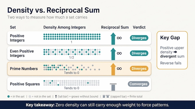
Ordinary density measures the fraction of integers belonging to a set. A divergent reciprocal sum measures something subtler: whether contributions across increasingly large scales accumulate without limit.
The primes illustrate the gap. Their density among all integers tends to zero, yet their reciprocal sum diverges. Squares are sparse too, but their reciprocal sum converges.
Erdős–Turán Conjecture: Comparing Integer Sets, Density, and Reciprocal Sums
| Set | Density Among Integers | Reciprocal Sum | Lesson |
|---|---|---|---|
| Positive Integers | 1 | Diverges | The harmonic series supplies the baseline |
| Even Positive Integers | 1/2 | Diverges | Positive density comfortably meets the condition |
| Prime Numbers | Tends to 0 | Diverges | Zero density can still carry sufficient weight |
| Positive Squares | Tends to 0 | Converges | Infinitude alone doesn’t meet the condition |
Every set of positive upper density has a divergent reciprocal sum. The reverse fails. That’s why the Erdős reciprocal sum conjecture reaches beyond positive-density theorems: it asks for patterns in sets that can occupy a shrinking fraction of the integers.
3. What Roth, Szemerédi, and Green–Tao Established
The history begins with a weaker question. Erdős and Turán’s 1936 work studied extremal progression-free sets and explicitly conjectured the three-term positive-density statement. The stronger reciprocal-sum formulation came later.
Roth proved that positive-density sets contain three-term progressions. Szemerédi established the all-length positive-density theorem. Green and Tao proved that the primes contain arbitrarily long progressions, including an extension to subsets with positive relative upper density among the primes.
These results address different hypotheses. Szemerédi handles density among all integers. Green–Tao handles the special arithmetic setting of primes. Neither, by itself, establishes the reciprocal-sum assertion for every set of positive integers.
The three-term reciprocal-sum case was already known through quantitative work by Bloom and Sisask. Later three-term estimates became stronger still. OpenAI’s manuscript explicitly claims no improvement to the three-term exponent. Its proposed advance is a summable bound covering every fixed progression length.
4. The Previous Barrier: Density Bounds That Shrink Too Slowly
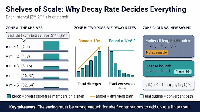
Define (r_k(N)) as the largest size of a subset of ({1,\ldots,N}) containing no nonconstant (k)-term progression.
Szemerédi’s theorem gives (r_k(N)=o(N)) for fixed (k). The proportion tends to zero, but that alone doesn’t settle the Erdős–Turán conjecture. The decay must be fast enough to satisfy
[ \sum_{m\ge1}\frac{r_k(2^m)}{2^m}<\infty. ]
Think of the intervals ([2^m,2^{m+1})) as shelves. Each shelf contains at most (r_k(2^m)) members of a progression-free set, and each contributes at most (2^{-m}). The question is whether the combined shelf contributions remain finite.
The manuscript contrasts its result with earlier all-length estimates saving a stretched exponential in (\log\log N). Those estimates don’t meet this summability requirement. Moving the saving to (\log N) changes the outcome.
The obstacle was quantitative control during iteration. Finding structured correlation is useful, but repeatedly restricting to structured regions can consume too much interval length and precision.
An elementary comparison shows why the decay rate matters. A shelf contribution bounded by a constant times (1/m) would still leave a divergent series. A bound by (1/m^{1+\delta}), with (\delta>0), would converge. The issue is therefore the cumulative contribution across scales, not simply whether individual contributions approach zero.
5. OpenAI’s Main Theorem: Quasipolynomial Bounds for Arithmetic Progressions
Theorem 1.1 states that, for every fixed integer (k\ge3), positive constants (C_k,c_k,\varepsilon_k) exist such that
[ r_k(N)\le C_kN\exp!\left[-c_k(\log N)^{\varepsilon_k}\right] \qquad(N\ge2). ]
Here (C_k) is a multiplicative constant, (c_k) controls the saving, and (\varepsilon_k) sets its stretched-exponential exponent. All may depend on (k), and the exponent isn’t optimized.
The equivalent density threshold says an (\alpha)-dense subset contains a progression when
[ \log N\ge A_k\bigl(2+\log(1/\alpha)\bigr)^{A_k} ]
for a suitable (A_k\ge1). “Quasipolynomial” describes the sufficient interval length as a function of inverse density. It doesn’t mean a polynomial-time algorithm for finding progressions.
These arithmetic progression density bounds beat every fixed inverse power of (\log N), eventually. They don’t give a fixed power saving in (N). That distinction is necessary because known progression-free constructions already rule out such a saving in the three-term case.
6. How Density Increments, Gowers Norms, and Nilsequences Fit Together
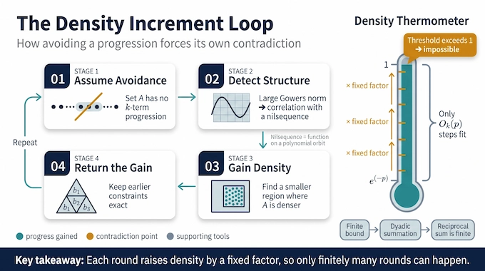
A density increment argument begins by assuming that a set avoids the desired progression. That avoidance forces detectable structure. The proof uses the structure to locate a smaller region where the set occupies a larger proportion.
Gowers norms measure the higher-order correlations relevant to longer progressions. An inverse theorem turns a sufficiently large norm into correlation with a nilsequence: a function evaluated along a polynomial orbit on a compact nilmanifold.
The manuscript uses the quasipolynomial interval inverse theorem of Leng, Sah, and Sawhney. It also relies on a radius-sensitive almost-periodicity theorem of Schoen and Sisask. These existing inputs are substantial parts of the mathematical foundation.
The new argument must convert correlation into a positive density gain at an affordable cost. Shift comparison lowers the degree of the tests while permitting multiplication by translated nonnegative functions. Positive counting and relative lifting then produce an absolute increment on an integer box.
Here “absolute” refers to the starting increment mechanism before returning to the constrained cell. The return requires separate estimates. A successful local gain isn’t yet an iterable proof.
7. Triangular Polynomial Cells: Keeping Earlier Constraints Intact
The manuscript organizes its regions as triangular polynomial cells. A spatial integer variable (u) determines integer blocks (b_1,\ldots,b_D) successively through narrow polynomial constraints:
[ \left|b_h-C_h(u,b_1,\ldots,b_{h-1})-\ell_h\right|_\infty \le w_h. ]
The block (b_h) has weight (h), and (C_h) has weighted degree at most (h). The depth (D) depends only on the fixed progression length. Narrow residual widths make each determining integer block unique when it exists.
Each block depends on the spatial variable and earlier blocks. Later constraints retain the earlier integer values exactly. An approximation that changes one block could corrupt every subsequent polynomial using it.
Theorem 2.1 supplies the triangular increment. It raises the certified density threshold by a fixed factor while retaining the determining data through exact integer reparametrizations.
Its decisive restriction concerns precision. Writing (Q_h=\log(2/w_h)), the additional precision at weight (h) depends on higher-weight precision budgets, not on the current (Q_h) or lower ones. This descending dependence prevents costs from feeding back into themselves indefinitely.
Weighted degree records the cost of variables with different weights. For example, (u^2) and a weight-two coordinate both have weighted degree two. This bookkeeping lets the proof add equations while retaining a fixed hierarchy, even as the number of coordinates grows.
8. Constrained Sampling and Rank Cuts Preserve Structure
Sampling makes a complicated cell accessible through parameter boxes, but ordinary sampling can destroy the constraints that define it. Section 3 builds constrained paths with comparison and detection guarantees suited to these regions.
Section 4 prepares cells through rank cuts. When a polynomial relation fails the required rank condition, the argument reorganizes the determining data while preserving the box certificate. Preparation can include copying higher-weight blocks into lower-weight blocks.
Rank conditions provide control over the relations encountered by the sampler. They support the comparison estimates needed to carry information between the sampled representation and the original region.
Section 5 tackles another danger: a cell may have extremely small mass. Detection estimates that deteriorate with the current layer’s width would ruin the recurrence. The proof uses densification to replace sparse factors by bounded ones before applying inverse theory, obtaining the required independence from that layer’s chart mass.
This is where the precision architecture earns its keep. The sampler must reveal useful structure without charging the proof repeatedly for every previously narrowed constraint.
9. Returning the Increment Through Passive and Active Layers
Section 6 transfers the density certificate to terminal boxes and obtains an increment there. Sections 7 through 9 return that gain to a region suitable for the next round.
At passive layers, where the testing degree is below the layer weight, comparison and scalar-transfer arguments move the information back through the existing structure. At active layers, the proof must handle more substantial polynomial interactions.
Section 8 globalizes the active-layer construction while retaining an exact marked projection onto the old equations. This allows additional structure without discarding the constraints inherited from previous rounds.
Section 9 extracts parameters and restores the next cell. It removes auxiliary flags, solves inactive equations, controls boundary losses, and eliminates the full active modulus. The output must again meet the theorem’s prescribed dimension and width recurrences.
The certificate compares the set’s mass inside a strict cell against a slightly enlarged cell’s mass. Keeping both versions controls boundary effects during restriction and restoration. Without that bookkeeping, an apparent gain could reflect a changed boundary rather than a usable increase in density.
The governing requirement is simple to state: the higher density found in a sampled representation must survive translation back into the original variables. Most of the technical difficulty lies in making that statement quantitatively reliable.
10. How Repeated Increments Produce the Final Bound
Section 10 closes the argument by scheduling the dimensions and precision budgets. Structural forecasts come first. Numerical precision is then chosen using those forecasts, working downward through the fixed number of weights.
For starting density roughly (e^{-p}), only (O_k(p)) fixed-factor increments can occur before the certified threshold exceeds one. A function bounded by one cannot satisfy such a certificate.
If the initial interval exceeds the scheduled requirements, the process has enough room to reach the impossible threshold. Therefore a progression-free set’s starting density must satisfy the claimed bound.
The triangular recurrences keep the total logarithmic loss polynomial in (p). A recurrence depending on every current precision could instead increase its effective polynomial degree at each round. The paper’s organizing achievement is controlling that cumulative cost.
11. From the Density Bound to the Reciprocal-Sum Proof
Once Theorem 1.1 is available, Corollary 1.2 follows by dyadic summation. If (A) avoids a fixed (k)-term progression, then
[ \sum_{a\in A\cap[2^m,2^{m+1})}\frac1a \le2^{-m}r_k(2^m) \le C_k e^{-c_k(m\log2)^{\varepsilon_k}}. ]
The right-hand side is summable in (m). Eventually it decays faster than (m^{-2}), because every positive power of (m) outgrows (\log m). The total reciprocal sum is finite, contradicting divergence. Applying this for each fixed (k) gives every finite length.
This is the bridge completing the manuscript’s Erdős–Turán conjecture proof. The hard work delivers the finite-set bound. The final infinite-set deduction is short enough to inspect directly.
Section 11 goes further. Corollary 11.2 provides a uniform harmonic bound (H_k) for every (k)-term-progression-free set. Corollary 11.4 permits the stronger hypothesis
[ \sum_{a\in A}\frac{(\log(2+a))^B}{a}=\infty ]
for any fixed (B\ge0). Larger weights make divergence easier, so this reaches additional sparse sets. Corollary 11.3 treats certain stretched-exponential weights for fixed (k), and Corollary 11.5 bounds harmonic tails.
The bounds also recover Green–Tao’s dense-primes conclusion. However, the manuscript doesn’t provide a practical numerical value of (H_k), or an optimized threshold for finding a specified progression.
12. What the Proof Establishes, What Lean Covers, and What Comes Next
As of October 11, 2026, OpenAI’s published scope note says the Lean formalization proves the reciprocal-sum conclusion for every requested length, with positive common difference. It explicitly excludes the manuscript’s quantitative extremal bound from that selected statement.
The distinction prevents a misleading shortcut. Formal verification of the Erdős–Turán conjecture’s qualitative conclusion doesn’t automatically verify Theorem 1.1, the stated parameter losses, or every weighted consequence by the same route.
The linked comparator challenge contains a placeholder proof because it specifies the target statement for comparison. It should be read alongside the repository’s verification instructions, rather than treated as the completed formal proof itself. OpenAI also describes the wider collection as containing results at different verification stages.
For readers assessing the OpenAI Erdős conjecture proof, the useful questions concern exact theorem coverage, the return argument’s dependencies, and whether the written quantitative proof survives detailed scrutiny. The remaining quantitative questions include explicit constants, practical thresholds, and optimal exponents.
The result’s significance lies in connecting sparse-set arithmetic to an iteration whose accumulated costs remain controlled. That connection is the heart of the proposed advance on the Erdős–Turán conjecture.
To understand the result, start with the finite-set bound, follow the summation argument, and check the scope of the formal verification. Follow Binary Verse AI for research explainers that track the mathematical claim, the evidence behind it, and the questions still worth asking.
1. Did OpenAI solve the Erdős–Turán conjecture?
OpenAI’s September 23, 2026 paper presents a proof of Erdős’s conjecture on arithmetic progressions. It establishes a quasipolynomial density threshold implying that any set of positive integers with a divergent reciprocal sum contains arithmetic progressions of every finite length. Independent assessment of the full 198-page argument remains important.
2. What is the Erdős–Turán conjecture in simple terms?
It states that if the reciprocals of the numbers in a set add up to an infinite sum, the set must contain arbitrarily long arithmetic progressions. For example, an arithmetic progression is 3, 7, 11, 15, where consecutive terms differ by four. The conjecture applies even to sets that become increasingly sparse.
3. Why didn’t Szemerédi’s theorem already prove the conjecture?
Szemerédi’s theorem guarantees arbitrarily long arithmetic progressions in sets of positive upper density. Erdős’s conjecture allows much sparser sets, including sets of zero density. Earlier general density bounds were insufficient to establish the necessary convergence of reciprocal sums for progression-free sets.
4. What is the main breakthrough in OpenAI’s proof?
The proof constructs density increments using triangular polynomial cells that preserve previous structural constraints while controlling accumulated losses. This produces a bound of the form \(r_k(N)\le C_kN\exp[-c_k(\log N)^{\varepsilon_k}]\) for every fixed \(k\ge3\), strong enough to derive the reciprocal-sum conclusion.
5. Has OpenAI’s Erdős–Turán proof been formally verified?
OpenAI publishes Lean formalization code for the reciprocal-sum conclusion, including a theorem in Results/Conclusions.lean. Its documentation distinguishes that conclusion from the paper’s stronger quantitative bound, which is outside the stated formalization scope. The code should not be presented as independent verification of every quantitative estimate in the paper.