

A graph can give every vertex exactly two selected connections and still leave you going around several separate loops. Getting one loop through the entire graph is the hard part. For decades, that distinction has kept a deceptively simple mathematical question open.
Barnette’s Conjecture asks whether every cubic, bipartite, planar, 3-vertex-connected graph contains a Hamiltonian cycle, a closed route through every vertex exactly once. OpenAI’s September 24, 2026 manuscript claims a proof of the full statement. Released with its October 6 mathematics announcement, the paper has a corresponding Lean formalization listed in the repository.
The surprising ingredient is a complex-valued sum designed to make unwanted configurations cancel. Another argument prevents the whole sum from disappearing. What survives supplies the structure needed for the cycle.
Original Research Paper: Paired States and Hamiltonian Cycles in Cubic Bipartite Planar Graphs (PDF)
Table of Contents
1. What Is Barnette’s Conjecture? A Simple Graph Example
A graph consists of vertices connected by edges. Barnette’s Conjecture concerns a specific class, with four conditions that work together.
The cube makes the claim tangible. Label its corners with three-bit strings. One Hamiltonian cycle is:
000 → 001 → 011 → 010 → 110 → 111 → 101 → 100 → 000
Consecutive strings differ in one bit, so each step follows an edge. Every corner appears once before the return.
A Hamiltonian cycle visits vertices. An Eulerian cycle uses every edge exactly once. Confusing them changes the problem completely.
2. Did OpenAI Solve the Conjecture? What the Evidence Shows
The manuscript states the full theorem. There’s no maximum number of vertices and no upper limit on face length.
For readers searching whether Barnette’s Conjecture is solved, the clearest answer is that OpenAI has published a claimed full proof and lists a formalization of that statement. Independent reproduction and mathematical review remain distinct questions.
One source of confusion is a challenge file containing Lean’s sorry, which marks an unproved statement. In a comparator setup, the challenge specifies the target while a separate module supplies the solution.
That placeholder alone establishes neither success nor failure. A useful verification report identifies the solution, checks its assumptions, and reproduces the comparison.
3. Why the Problem Resisted Proof for Decades
Recorded in 1969 and attributed to David Barnette, the conjecture belongs to a history of attractive statements about Hamiltonian cycles that proved unexpectedly fragile.
Tait’s earlier conjecture concerned cubic polyhedral graphs, without requiring bipartiteness. Tutte disproved it in 1946. Barnette’s formulation keeps planarity and 3-connectivity while adding the bipartite condition.
Researchers established important restricted cases. Goodey handled graphs whose faces are quadrilaterals or hexagons. Feder and Subi allowed larger faces within a controlled face-coloring structure. Schnieders later established the faces-at-most-eight case. The related Barnette–Goodey result proved by Kardoš has different hypotheses and shouldn’t be mistaken for the full target.
The stubborn issue is global connectedness. In a cubic bipartite graph, a perfect matching leaves two edges at every vertex when removed. Those remaining edges form cycles, but potentially several.
Locally, each vertex looks satisfied. Globally, the route may be useless. A proof must control how the entire structure fits together, rather than merely ensure that every vertex has the right degree.
4. The Dual-Graph Idea: Turn the Cycle Problem Into Two Trees
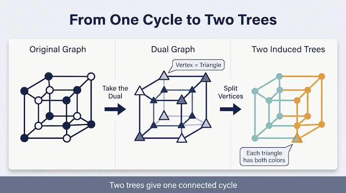
The proof changes the viewpoint before attempting the difficult step.
Draw the original graph on a sphere. Put a new vertex inside each face, then connect two new vertices whenever their faces share an edge. This creates the dual graph.
Because the original graph is cubic, each original vertex corresponds to a triangular dual face. Its bipartition colors those triangles black and white, with opposite colors on either side of every edge.
An established equivalent formulation asks for a partition of the dual’s vertices into two sets, each inducing a tree. An induced tree contains every edge between vertices in its set. You can’t discard an inconvenient internal edge and still claim inducedness.
Why does this help? Each triangular face must contain vertices from both sets. Exactly one of its edges then lies within a set. The other two cross between sets and correspond to two selected edges at the original vertex.
That supplies degree two everywhere. The tree structure supplies the missing global control needed to make those edges one connected cycle.
5. Paired States: The Matching Structure Behind the Proof
First consider a dual triangulation with no separating triangle, meaning no three-edge cycle has vertices strictly on both sides.
Choose a black triangle as the outer face. Its three vertices become roots. The remaining black triangles and the vertices outside those roots have equal counts.
A state matches each remaining black triangle to one incident nonroot vertex, using every nonroot exactly once. A paired state consists of two such assignments, called $r$ and $s$, choosing different vertices at every triangle.
The paper establishes existence through a planar counting inequality and an integral network flow. Capacities enforce two assignments per triangle and per nonroot, with no shared incidence. The resulting degree-two bipartite structure splits into two perfect matchings.
This step provides compatible pairs to work with. It doesn’t yet guarantee the desired forest. For the second state $s$, select the edge opposite its chosen vertex in every remaining black triangle. Call that edge set $Q_s$. The next task is to ensure that $Q_s$ contains no cycle.
6. The Disk Identity That Makes Cancellation Possible
The proof needs a dependable relationship between geometry and signs.
Give a directed edge weight $+1$ when its black face is on the left, and $-1$ when that face is on the right. Reversing an edge reverses its sign.
For particular directed cycles produced from a state, the total signed weight is always $-3$ counterclockwise and $+3$ clockwise.
The exact magnitude comes from counting black faces, white faces, interior vertices, and boundary edges inside the cycle. Euler’s formula constrains the disk. The state’s bijection supplies another constraint, fixing how black faces match interior and boundary vertices.
That matching condition is essential. The identity doesn’t apply to an arbitrary loop drawn through the triangulation.
The payoff is predictable phase behavior. Once divided by three, each eligible cycle contributes $+1$ or $-1$ to an exponent. Its orientation therefore determines a factor of $i$ or $-i$, where $i^2=-1$.
7. OpenAI’s Complex-Number Trick: Cancel Bad Configurations
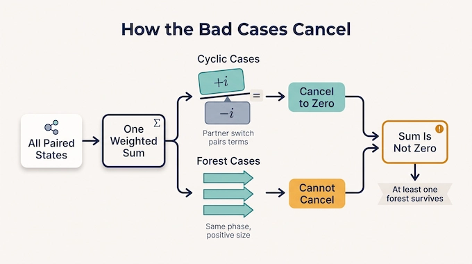
This proof of Barnette’s Conjecture organizes all paired states into one finite weighted sum:
[ Z(x)=\sum_{(r,s)} i^{J(r,s)}e^{x\omega(s)}. ]
Here $J$ is the signed edge sum divided by three. The real weight $\omega$ depends only on the second state, and $x$ is a real parameter.
First, fix a second state whose opposite-edge set $Q_s$ contains a cycle. The paper constructs a partner-switching operation that reverses that cycle through changes to $r$. Applying it twice returns the original pair, and no pair is left unmatched.
The disk identity makes the exponent change by two in magnitude. Since $i^{J+2}=-i^J$, paired terms have opposite phases. Their real weights agree because $s$ hasn’t changed.
Every contribution associated with a cyclic $Q_s$ cancels.
But cancellation alone could leave zero.
The second evaluation groups pairs by the undirected cycles formed by joining their two choices in each triangle. Each cycle can be oriented independently.
The proof adds spokes from triangle centers to their vertices and assigns weights with positive circulation around every counterclockwise spoke cycle. This makes the two orientations have strictly different real weights.
Each cycle’s grouped contribution vanishes to first order at $x=0$. Groups with the fewest cycles therefore contribute at the lowest occurring Taylor order. Crucially, those leading terms have the same complex phase and positive magnitudes. They can’t cancel one another.
Thus $Z$ isn’t identically zero. Since all cyclic $Q_s$ contributions disappeared, at least one forest configuration must remain.
8. How a Surviving Forest Produces One Hamiltonian Cycle
The forest $Q_s$ has three components, each containing exactly one root. The paired state provides an orientation in which every nonroot has one outgoing edge and roots have none. Counting edges in each tree forces that root distribution.
The paper then builds an incidence graph using triangle centers and spokes. The forest, together with the outer triangle’s three spokes, becomes a spanning tree in that graph.
A standard planar duality fact says that edges complementary to a spanning tree form a spanning tree in the dual. Here, that produces a tree on the white triangles.
Rooting this tree determines one selected edge at every black and white face. Another disk-identity argument proves that the selected edge set is acyclic.
Its complementary dual is connected and has degree two at every vertex. A finite connected graph with that degree pattern is one cycle, completing the central construction.
Separating triangles require one final step. The triangulation is split into smaller pieces, and a prescribed local pattern makes their two-tree partitions agree on the shared triangle. Corresponding trees meet in a vertex or an edge, so gluing preserves their tree structure.
That extends the construction to the full class.
9. Why the Proof Looks Like Physics and What Is Actually New
The online excitement centers on this cancellation mechanism. In the Hacker News discussion, Jake Boggan described working on the conjecture for years and finding the complex-valued argument striking. Reddit discussions picked up the resemblance to techniques from physics.
The analogy is understandable. Physics often packages many configurations into weighted sums, where phases control cancellation and parameters help isolate contributions.
The manuscript itself acknowledges relevant mathematical ancestry. Its assignments are related to Tutte states. The passage between matchings and trees connects with Temperley’s correspondence. Grouping two matchings by their union cycles is familiar from the double-dimer model.
Those connections explain why the proof feels broader than an elementary graph argument. They don’t establish that a quantum computer was used or that renormalization supplied the solution.
The claimed contribution lies in making these structures work together through the fixed-second-state cancellation and positive-circulation argument.
Established ingredients can produce a genuinely new proof when their combination crosses a previously unresolved barrier. Determining the exact extent of that novelty requires a careful literature comparison.
10. Why the Result Matters for Graph Theory and Algorithms
Barnette’s Conjecture matters because it identifies conditions guaranteeing a global cycle despite unrestricted graph size and face length.
The manuscript also records consequences beyond basic existence. Given any single edge in a qualifying graph, there is a Hamiltonian cycle avoiding it. Through an established equivalence, it derives a prescribed-path result for finite simple cubic, 3-vertex-connected, Pfaffian bipartite graphs.
In that broader class, every three-edge path lies within a Hamiltonian cycle. Pfaffian structure concerns special orientations relevant to perfect matchings, and the class includes some nonplanar graphs.
For developers, the boundary is equally important. The paper explicitly gives no polynomial-time construction guarantee. Its finite exponential sum establishes existence without promising an efficient procedure for finding the surviving state.
A max-flow component doesn’t make the entire argument efficient.
Nor does this solve traveling-salesperson optimization. A Hamiltonian cycle concerns visiting every vertex along existing edges. Finding the cheapest tour adds an optimization objective.
The practical research opportunity is to investigate whether the proof’s existence argument can become an efficient construction. Until then, claims of faster logistics software or network routing would run ahead of the evidence.
11. What Barnette’s Conjecture Reveals About AI Research
The published method provides something concrete to inspect. It isn’t simply a list of tested graphs. However, the final proof doesn’t reveal every search step, failed attempt, or resource used during discovery. Labeling that unseen process “brute force” explains little without defining what was searched.
OpenAI attributes the release to an internal frontier model. Its announcement reports average compute equivalent to roughly three hours of ChatGPT Pro thinking per result. That is neither a Barnette-specific duration nor a promise that an ordinary ChatGPT session can reproduce the discovery.
The human implications deserve care, too. Researchers can feel both excitement about a solution and loss when a longstanding personal project changes overnight.
There is still substantial work in understanding, checking, simplifying, and extending the argument. This paper’s finite cancellation mechanism is explainable, even if a full audit requires specialist knowledge.
A successful proof would strengthen the case for AI-assisted mathematical discovery. It wouldn’t, by itself, establish consciousness, recursive self-improvement, or a timetable for replacing researchers.
12. The Next Step Is to Understand the Mechanism
The most useful lesson from Barnette’s Conjecture is the proof’s architecture. Local matching constraints create candidate structures. A disk identity controls their phases. Cancellation removes unwanted cycles, and nonvanishing guarantees a survivor. Planar duality then turns that survivor into the required route.
For readers, start with the cube example and follow what each step establishes. For builders and researchers, inspect the formal target, seek reproducible verification, and ask whether the existence argument suggests a usable algorithm.
Explore more research-paper explainers at Binary Verse AI, and follow how AI-generated mathematical ideas become understood, verified, and extended.
1. What does Barnette’s conjecture say?
Barnette’s conjecture says that every finite simple graph that is cubic, bipartite, planar, and 3-vertex-connected has a Hamiltonian cycle—a closed route visiting every vertex exactly once before returning to the start. The cube graph is a familiar example satisfying all four conditions.
2. Has OpenAI proved Barnette’s conjecture?
OpenAI’s manuscript claims a proof of the full conjecture, without restricting graph size or face length. Its repository also describes a Lean formalization covering the full statement. That published evidence should be distinguished from an independently reproduced formal check and expert review.
3. How does OpenAI’s proof use complex numbers?
The proof assigns complex phases to paired graph configurations. Configurations containing unwanted cycles cancel in opposite-phase pairs. A second argument shows that the total weighted sum cannot vanish, forcing a surviving forest configuration. Planar duality then turns that structure into a Hamiltonian cycle. This is a mathematical cancellation argument.
4. Does the proof give a fast algorithm for finding Hamiltonian cycles?
The manuscript explicitly gives no polynomial-time construction guarantee. Proving that every graph in this class contains a Hamiltonian cycle does not establish an efficient way to find it, solve the general Hamiltonian-cycle problem, or optimize a traveling-salesperson tour.
5. Did AI invent an entirely new method or combine existing mathematics?
The paper combines established ideas—including planar duality, matchings, and state constructions—with its weighted cancellation and nonvanishing argument. It acknowledges related earlier methods. The important question is whether this combination establishes the previously unresolved theorem; assessing its precise originality requires comparison with the mathematical literature.