
Introduction
If you have ever watched a large run go sideways at 3 a.m., you know the weird part is not the failure. The weird part is how sudden it is. Loss looks fine, gradients look normal, then a small architectural “improvement” turns into a fireworks show.
That is the vibe behind DeepSeek mHC. It is not a paper that shows up to brag about a massive benchmark jump. It shows up to fix a fragile scaling trick, then quietly asks a bigger question, what if width in the residual stream is a real scaling knob, not a hack you pray over.
In one sentence, DeepSeek mHC takes the “Hyper-Connections” idea, keeps the good part (a wider residual stream with learnable mixing), then clamps the mixing so it behaves like an identity map across depth. The authors also treat systems work as first-class, because stability without speed is just a science project.
Table of Contents
1. DeepSeek mHC In 60 Seconds
Here is the short version you can keep in your head.
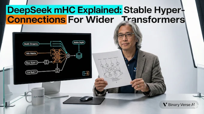
Hyper-Connections widen the residual stream from C ton×C and learn how to mix those streams using a matrix inside the residual pathway. That buys representational capacity without paying the usual FLOPs bill, which is why people got excited in the first place.
The catch is the residual “identity mapping” is not just a cute ResNet tradition. It is the stability rail. When the mixing is unconstrained, composing it across many layers stops behaving like identity, and signals can explode or vanish. The paper shows exactly that failure mode, including a sharp loss surge around ~12k steps and extreme amplification metrics peaking around 3000.
DeepSeek mHC fixes this by projecting the residual mixing matrix onto the manifold of doubly stochastic matrices (the Birkhoff polytope), enforced in practice with the Sinkhorn–Knopp algorithm. That makes the residual mixing non-expansive and compositional across depth, while still allowing “lane changes” between streams.
And because the real bottleneck in modern LLM infrastructure is often memory movement, not math, the paper spends serious effort on kernel fusion, mixed precision, recompute, and pipeline overlap, reporting just a 6.7% training-time overhead at expansion rate n = 4.
Table 1. Architecture At A Glance (The Parts That Matter)
DeepSeek mHC Architecture At A Glance
| Piece | What Changes | Why It Helps | What Could Break |
|---|---|---|---|
| Wider residual stream (n streams) | Residual width goes from C to n×C | Adds capacity without scaling layer FLOPs | Extra memory traffic, bigger activation footprint |
| Learnable residual mixing | Streams can exchange information each layer | Better feature fusion across depth | Unconstrained mixing compounds, can destabilize training |
| Manifold constraint | Residual mixing is forced to stay “well-behaved” | Preserves stable propagation while still mixing | Adds constraint enforcement cost, needs efficient kernels |
| Systems optimizations | Fusion, recompute, overlap | Keeps the idea deployable | Without it, you hit the GPU memory bandwidth bottleneck hard |
Tip: If columns feel tight on mobile, swipe sideways inside the table area, the page itself will not scroll horizontally.
2. The Real Problem: Width Is The Missing Scaling Knob
Most scaling talk reduces to two dials: more compute, more LLM training data. Sometimes we add a third dial, better data quality. But architecture has its own dials, and the Transformer’s default residual pathway is oddly conservative: a single stream, mostly an express elevator that keeps gradients alive.
Hyper-Connections argue that this is leaving performance on the table. If the residual stream is a highway, why force everything into one lane?
The paper makes the point crisply: because the expansion rate n can be small compared to C (think n = 4), the added compute can be negligible, which makes residual width feel like a “cheap” way to scale.
That is an architectural promise with real implications for AI scaling laws. If you can increase effective capacity without paying proportional FLOPs, you are changing the shape of the compute-quality curve, at least locally.
3. Residual Connections: The Identity Trick That Keeps Training Boring
The original residual connection is simple: output equals input plus a learned residual function. The important part is not the plus sign, it is the “input goes through untouched” property. Across many layers, you can write the deep representation as the shallow representation plus a sum of residuals. The identity path is the stable backbone.
This is why “Hyper-Connections vs residual connections” is not a cosmetic comparison. Residuals are a stability contract. If you mess with the identity behavior, you need to replace that contract with something equally strong.
4. What Hyper-Connections Tried To Do, And Why It Blows Up
Hyper-Connections expand the residual stream and introduce learnable mappings: a “pre” map to compress the widened stream into the layer input, a “post” map to write the layer output back into the widened stream, and a residual mixing matrix that blends the streams.
The core issue is compositional. A single unconstrained mixing matrix might look harmless. Multiply a lot of them together across depth and you get a composite transformation that can amplify or damp signals wildly. The paper spells it out: the composite mapping fails to preserve the global mean, leading to unbounded signal amplification or attenuation and training instability at scale.
Empirically, the failure looks like what practitioners fear: loss surge, gradient norm instability, and amplification metrics that go off the rails. The reported Amax Gain Magnitude peaking around 3000 is the kind of number that makes you stop blaming your optimizer.
This is the part where DeepSeek mHC earns its keep. It does not argue that Hyper-Connections were “wrong.” It argues they were under-constrained.
5. DeepSeek mHC: The Key Idea, Explained Like A Human

Picture n parallel residual “lanes.” Hyper-Connections let you mix lanes freely with a learnable matrix. DeepSeek mHC says, mix lanes all you want, but the mixing must behave like a conservation law.
Concretely, it constrains the residual mixing matrix to be doubly stochastic: non-negative entries, each row sums to 1, each column sums to 1.
Why that specific constraint?
- Norm preservation: the spectral norm is bounded by 1, so the mapping is non-expansive. That directly targets gradient explosion.
- Compositional closure: multiply doubly stochastic matrices together, you stay in the set. That means the “identity-like” behavior survives depth.
- Geometric meaning: the set is the Birkhoff polytope, the convex hull of permutation matrices. Intuitively, your residual mixing becomes a soft blend of permutations, a controlled way to shuffle and fuse streams over depth.
That is the “Manifold-Constrained Hyper-Connections” part, and it is a nice example of constraint design that feels more like engineering than aesthetic math.
6. Why “Doubly Stochastic” Prevents Blow-Ups
Let’s keep it practical. If each row sums to 1, then each output stream is a convex combination of input streams. If entries are non-negative, you do not get cancellation games where large positives and negatives fight each other and amplify numerical noise.
Also, because the set is closed under multiplication, you do not get the “quiet drift” where each layer nudges the residual mapping away from identity until the whole model becomes a signal amplifier.
This is the real philosophical difference. Hyper-Connections add expressive routing. DeepSeek mHC adds a routing constitution.
7. Sinkhorn–Knopp In Practice: Constraint Enforcement Without Drama
A constraint is only as good as its implementation. The paper applies the Sinkhorn–Knopp algorithm to project the residual matrix onto the doubly stochastic manifold. It exponentiates to make entries positive, then alternates row and column normalization until convergence.
They pick a practical iteration count, tmax = 20, rather than chasing infinity.
This is also where DeepSeek mHC makes a subtle move: it uses sigmoid-based constraints for the input and output mappings too, keeping them non-negative to avoid destructive cancellation.
8. Results That Matter: Stability First, Then Real Gains

If you only care about leaderboards, you will read this section and shrug. The gains are not the point.
For the 27B setup, the paper reports that the constrained variant mitigates the instability seen in HC and reaches a final loss reduction of 0.021 compared to baseline, with gradient norms staying stable and comparable to baseline behavior.
And yes, it translates into downstream improvements. Here is the table the paper provides, reproduced cleanly for quick scanning.
Table 2. Downstream Benchmarks (27B Models)
DeepSeek mHC 27B Benchmark Table
| Model | BBH (3-shot EM) | DROP (3-shot F1) | GSM8K (8-shot EM) | HellaSwag (10-shot Acc.) | MATH (4-shot EM) | MMLU (5-shot Acc.) | PIQA (0-shot Acc.) | TriviaQA (5-shot EM) |
|---|---|---|---|---|---|---|---|---|
| 27B Baseline | 43.8 | 47.0 | 46.7 | 73.7 | 22.0 | 59.0 | 78.5 | 54.3 |
| 27B w/ HC | 48.9 | 51.6 | 53.2 | 74.3 | 26.4 | 63.0 | 79.9 | 56.3 |
| 27B w/ mHC | 51.0 | 53.9 | 53.8 | 74.7 | 26.0 | 63.4 | 80.5 | 57.6 |
Tip: Swipe sideways inside the table area to see all columns on mobile, the page itself will not scroll horizontally.
The authors also call out that, compared to HC, the constrained approach improves reasoning benchmarks like BBH and DROP by a couple points.
That is not a revolution. It is a signal that the stability constraint did not neuter the expressivity.
9. Why The Systems Section Is Half The Paper

Now we get to the part that separates a nice idea from something you can actually train. Modern LLM training is often throttled by the “memory wall,” meaning memory access dominates runtime in key kernels. Wider residual streams multiply memory traffic, and naive implementations will slam straight into the GPU memory bandwidth bottleneck.
The paper does the unglamorous accounting: HC increases per-token memory access roughly proportional to n, and also inflates GPU memory footprint because intermediate activations of those mappings are needed for backprop.
They even provide a per-token I/O breakdown, showing how total reads and writes scale with n in the naive path. So DeepSeek mHC leans hard into optimization:
- CUDA kernel fusion and mixed precision: fuse shared-memory-access operations into unified kernels to reduce launch overhead and memory traffic.
- Bandwidth-aware fusion of residual application: fusing post and residual mappings with residual merge reduces reads from (3n + 1)C to (n + 1)C and reduces writes from 3nC to nC for that kernel path.
- Sinkhorn inside one kernel: implement the Sinkhorn–Knopp iteration in a single kernel, with a custom backward kernel that recomputes intermediates on-chip across the whole iteration.
- Recomputing: discard intermediate activations for the mHC kernels after forward pass and recompute them during backward, storing only block inputs.
This is exactly the stuff people forget when they ask “How to train LLM on your own data.” You can have pristine data, a good optimizer, and a clever architecture, and still get kneecapped by memory traffic and kernel launch overhead. At scale, LLM infrastructure is the product.
10. Communication Overlap And Distributed LLM Training Reality
Once you widen the stream, pipeline parallelism gets more expensive too. The paper points out HC can require n-fold more communication cost in pipeline parallelism, which increases bubbles and reduces throughput.
To deal with that, they extend the DualPipe schedule to overlap the extra work introduced by the constrained mappings.
This is the difference between a method that demos on a single node and one that survives Distributed LLM training.
And it backs up the headline: with these optimizations, the paper reports only 6.7% additional training-time overhead when n = 4.
11. Where This Fits In AI Scaling Laws
The paper frames residual width as an additional scaling dimension that complements compute and dataset size, not a replacement for them.
If you think in “frontier curves,” the promise is simple: you might get better quality at similar FLOPs because the residual pathway can carry and fuse more information.
The scaling experiments in the paper support the idea that the advantage holds as compute budgets rise, with only marginal attenuation at larger scale.
That is the responsible version of the claim. It does not say “new scaling law.” It says “new knob that seems to keep working as you scale.”
12. Practical Takeaways, And What To Watch Next
Here is the grounded verdict.
DeepSeek mHC is not a flashy new block like attention once was. It is closer to a structural reinforcement beam. The main win is that it turns a promising but unstable idea into something trainable, by restoring identity-like behavior with a constraint that composes cleanly across depth.
If you run large training jobs, this is the kind of paper you bookmark because it answers the annoying questions you actually have:
- What fails at scale, and how exactly does it fail?
- What constraint fixes it, and why does that constraint survive depth?
- What does it cost in real throughput, once you fight the memory wall?
If you are smaller-scale, the idea still matters, but the path is different. You probably will not implement a custom Sinkhorn backward kernel tomorrow. What you can do is watch for reference implementations that expose the constraint and let you test stability, even if you cannot replicate the full infrastructure stack.
What I want to see next is simple:
- Reproductions in other codebases and other model families.
- Larger expansion rates and a clearer map of where memory traffic becomes the limiting factor again.
- More evidence that residual width competes with, or complements, the usual tricks in LLM training like better data mixtures and better optimization schedules.
If you care about scaling, DeepSeek mHC is worth your attention because it treats architecture and systems as inseparable. That is the real lesson. Ideas do not scale, implementations do.
If you are building models, or even just tracking where the next efficiency gains come from, keep DeepSeek mHC on your shortlist.
Then do the most useful thing a reader can do: pull the paper up, skim the figures for the failure mode, skim the kernel section for the fix, and ask yourself which part of your own stack would break first if you widened the residual highway.
1) What is training in LLM?
LLM training is the process of updating model weights so it predicts the next token more accurately across massive datasets. It is usually dominated by large-scale pretraining, then optional fine-tuning and alignment for task behavior.
2) What is the basic training of an LLM?
The basic pipeline is: collect and clean LLM training data, tokenize it, pretrain with next-token prediction, validate on held-out sets, then fine-tune for tasks and align with preference or instruction data if needed.
3) How long does it take to train LLMs?
It depends on model size, tokens, GPUs, and efficiency. Smaller models can finish in days, frontier runs can take weeks to months. Architecture and LLM infrastructure improvements, including DeepSeek mHC-style stability and kernel work, aim to get more quality from the same budget.
4) How is LLM being trained?
Most LLMs use distributed LLM training with data parallelism plus model or pipeline parallelism on GPUs. Mixed precision, activation checkpointing (recompute), and aggressive kernel optimization are common because memory movement, not math, often sets the speed limit.
5) What is DeepSeek mHC (Manifold-Constrained Hyper-Connections)?
DeepSeek mHC is an architecture that widens the residual “information highway” into multiple streams, then constrains how those streams mix so training stays stable across depth. It targets the instability seen in unconstrained Hyper-Connections by enforcing well-behaved mixing (often described via doubly-stochastic constraints with Sinkhorn-Knopp).