Introduction
If you’ve ever tried to scale an RL run and felt like you were flying by instrument in a storm, you’re not alone. For years, Reinforcement Learning AI has delivered flashes of brilliance, then slipped into instability right when the stakes get high. The result, wasted compute and teams guessing which tweak will hold at scale. A new study changes that. Meta’s large, methodical investigation lays out scaling laws for RL that behave predictably, then packages the findings into a practical recipe called ScaleRL. The punchline, you can now forecast where your run will land and make principled choices about what to scale, not just cross your fingers and spend.
The core insight is simple to say and powerful in practice. Reinforcement Learning AI doesn’t follow the same power laws that govern pre-training. It follows a sigmoidal compute to performance curve with a clear ceiling and a clear slope. Fit that curve early, and you can forecast the finish. Do this with a stable training recipe, and you can scale to six figures of GPU hours with a level of calm usually reserved for pre-training teams.
If you care about reinforcement learning for LLMs, this is a welcome turn. We finally have a framework to judge algorithmic ideas without running every experiment to the endpoint. Better yet, the study backs the theory with a long run that hits 100,000 GPU-hours and lands right where the early fit said it would. Reinforcement Learning AI just got a forecasting tool.
Table of Contents
1. The Scaling Problem: Why RL Has Lagged Behind Pre-Training
Pre-training has long enjoyed tidy power laws. Add data and compute, get smooth gains. Reinforcement Learning AI never felt that way. Small nips to the loss, the off-policy setup, or the data curation could flip a result from promising to brittle. That made big runs a gamble, and the cost kept most teams out. The Meta study calls this out directly, noting that RL compute has surged across model families, yet a predictive methodology was missing, which stalled progress and forced ad-hoc recipes.
The team frames the question in practical terms. What should you scale first, and how soon can you trust the signal. That framing is the doorway to the new laws, and to a more efficient path for Reinforcement Learning AI.
2. A New Science Of Scaling: The Sigmoidal Curve For RL
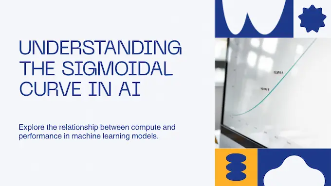
The paper models RL performance (on an iid validation set) as a saturating sigmoid in compute (C). There are three intuitive parameters, a ceiling (A), a slope (B) that captures predictive scaling efficiency, and a midpoint (C_{\text{mid}}). When you fit this curve early, you can extrapolate reliably to larger budgets. In other words, you can forecast the payoff of more GPUs. That is the missing science in Reinforcement Learning AI.
To show it’s not a toy, the authors take ScaleRL to 100,000 GPU-hours and confirm the forecast. The extrapolated curve, fit on the early portion, tracks the full run closely. The lesson, trustworthy curves beat anecdotal charts when the bill runs into six figures.
3. The Bitter Lesson Of RL: Why Early Performance Is Deceptive
The team repeatedly observes a pattern that has tricked many of us. Methods that look “fast” at low compute, for example tiny batches or short contexts, often hit lower ceilings. Methods that look “slow” initially can scale past them with a higher asymptote. Batch size is the clean illustration. Small batches may pop early, then stall downstream. Larger batches lift the final ceiling and avoid stagnation as compute grows. Long context shows the same story, slower start, higher destination. These are the exact traps the sigmoid fit avoids, because it separates efficiency from the ceiling. Reinforcement Learning AI needs that separation.
4. “ScaleRL”: A Proven, Best-Practice Recipe For Scalable RL
The study doesn’t stop at theory. It distills a stable, reproducible recipe that consistently lands on the predictable curve. ScaleRL combines an asynchronous setup, a robust loss, a precision fix where it matters, and a data curriculum that wastes less compute. Reinforcement Learning AI finally has a house style you can trust.
4.1 Asynchronous Setup: PipelineRL That Cuts Idle Time
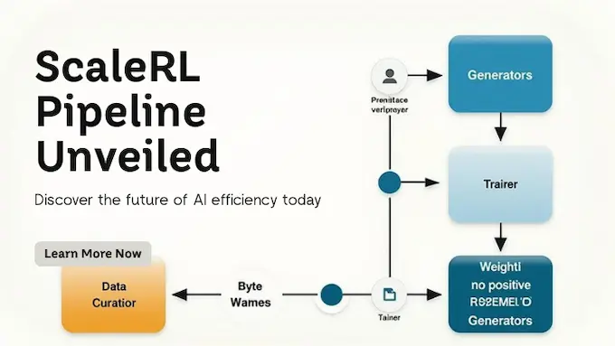
Classic asynchronous RL for language models often runs PPO in batches with stale rollouts. PipelineRL streams generations and pushes new weights to generators as soon as an update lands. That simple change tightens the feedback loop, improves the slope (B), and even nudges the asymptote (A). Meta compares PipelineRL-k to PPO-off-policy and finds similar ceilings with PipelineRL reaching the ceiling faster, because idle time drops and the training distribution stays closer to on-policy. This is why ScaleRL defaults to PipelineRL with k set to eight. It is an RL best practices choice, not a fad.
4.2 Loss And Precision: CISPO Plus An FP32 Head
Losses matter. The study finds CISPO outperforms DAPO on asymptotic reward and maintains a steadier improvement curve. Pair that with a surgical precision fix at the language model head, computed in FP32 for both generator and trainer, and you avoid numerical mismatches that blow up importance weights. The head-only FP32 change lifts the asymptote from 0.52 to 0.61. In short, the loss makes the climb cleaner and FP32 at the head locks in the destination. Reinforcement Learning AI benefits from both.
4.3 Data Curation: Filter What Teaches You Nothing
Two data-side moves deliver free wins. First, drop zero-variance prompts inside the batch, since they contribute no gradient. Second, maintain pass-rate history and stop resampling prompts that the policy consistently aces. The study’s simple “no positive resampling” rule removes prompts with pass rate at or above 0.9 in future epochs. Both steps lift the asymptote and improve stability. Reinforcement Learning AI loves compute spent on learning, not on padding.
4.4 ScaleRL In One Look
ScaleRL Components for Reinforcement Learning AI
| Component | Choice In ScaleRL | Primary Effect | Why It Matters |
|---|---|---|---|
| Asynchronous Setup | PipelineRL, k = 8 | Higher slope (B), slightly better (A) | Reduces idle time and keeps training close to on-policy. |
| Loss Type | CISPO | Higher asymptote (A), steadier curve | More robust than DAPO across settings. |
| Precision | FP32 at LM head | Increases (A) from 0.52 to 0.61 | Fixes generator, trainer numeric mismatch. |
| Loss Aggregation | Prompt-level | Best asymptotic performance | Treats each prompt fairly. |
| Advantage Norm | Batch-level | Stable, slightly better overall | Good theory, solid practice. |
| Data Filtering | Zero-variance drop | Higher (A) | Don’t learn from non-signals. |
| Curriculum | No-positive resampling | Higher (A) | Stop over-training solved prompts. |
Scaling Axes for Reinforcement Learning AI
| Scaling Axis | Early Behavior | Long-Run Outcome | Practical Read |
|---|---|---|---|
| Batch Size | Small looks better early | Large wins with higher (A) | Prefer larger batches for downstream stability. |
| Context Length | Short moves quickly | Long lifts the ceiling (A) | Budget for longer contexts when chasing max performance. |
| Model Size | Bigger is steadier than you think | Larger MoE beats dense with less RL compute | Scale model and compute in tandem. |
| Gens Per Prompt | Minimal effect at fixed total batch | Curves mostly unchanged | Tune elsewhere first. |
5. How To Predict The Future: Extrapolating From Small-Scale Runs

Here’s the workflow I recommend. Run reinforcement learning an introduction of your recipe at half your target compute, fit the sigmoid, then extrapolate. If the curve predicts a strong finish, scale with confidence. The team does this across axes and recipes and sees clean fits that match extended training, including in a 100,000 GPU-hour run. This is predictive scaling in practice, not in theory. Reinforcement Learning AI finally has a way to estimate the finish line early.
They also apply leave-one-out tests. Start with ScaleRL, revert exactly one choice, and watch how the slope and ceiling shift. Most variants end up at similar ceilings, yet lose efficiency, which shows up as a smaller (B) after transforming the sigmoid into a log-log form. That analysis tightens your decision-making. When two options tie on asymptote, pick the one with the steeper slope. Reinforcement Learning AI moves faster when the slope is yours.
6. The Impact On Real-World AI: Unlocking The Path To Capable Agents
Why does this matter beyond pretty curves. Because AI agent training lives or dies on confidence in the next dollar of compute. If a team knows that 50,000 GPU-hours delivers a predictable boost and that 100,000 will land at a forecasted score, planning gets sane. The study makes this argument explicit by showing stable extrapolations from early points to the full 100,000 GPU-hour run, with downstream gains that generalize to tougher benchmarks. Reinforcement Learning AI stops being a black box and starts being a roadmap.
That opens the door for broader, more realistic environments. If your goal is an assistant that navigates tools, desktops, or browsers, you can budget the scale-up and choose scaling knobs with purpose. Longer context when you need the ceiling. Larger batches when you need downstream stability. Bigger models when you can afford the jump. This is the difference between a moonshot and an engineering program. It’s what Reinforcement Learning AI has been missing.
7. What This Means For The Open-Source Community
The democratizing angle is real. The paper doesn’t just publish plots. It publishes a recipe that small labs can adopt, along with a standard curve-fitting protocol. You can test a new loss or a data trick at modest scale, fit the sigmoid, and estimate whether it scales. That lets the community prune dead ends without burning 100k GPU-hours every time. The authors also highlight that while many LOO variants tie on asymptote, ScaleRL stays the most efficient. That gives open teams a sane default to build on. Reinforcement Learning AI advances faster when we stop guessing.
8. Practical Playbook: Decisions That Matter And Why
Think of your choices in three buckets.
8.1 Decisions That Shift The Ceiling
Longer context and larger models lift (A). If your product needs a new level of reasoning depth, push here. The data shows 32k token runs eventually surpass short-context runs despite a slower start, and that a 17B×16 MoE can outperform an 8B dense model with far less RL compute. This is where Reinforcement Learning AI trades short-term speed for destination quality.
8.2 Decisions That Improve Efficiency
Asynchronous setup and the right loss improve (B). PipelineRL reaches the ceiling faster than PPO-off-policy, and CISPO gives a cleaner climb than DAPO. Precision at the head, small change, big effect. If you need to hit a milestone inside a fixed budget, optimize here. This is what good RL best practices look like.
8.3 Decisions That Avoid Wasted Compute
Drop zero-variance prompts. Stop resampling solved prompts. Use prompt-level aggregation so each task speaks with the same volume. Use batch-level advantage normalization for a steady signal. These changes add up. They raise (A) and reduce variance across runs. They also make Reinforcement Learning AI cheaper to trust.
9. Conclusion: The “Art” Of Scaling RL Is Now A Science
The field asked for a way to scale RL with the same confidence as pre-training. This work delivers a principled curve, a tested recipe, and the evidence that early fits forecast long runs. The central move is decoupling efficiency from the ceiling, then designing the training stack to lift both. Reinforcement Learning AI gets a language for trade-offs and a playbook to act on them. The unpredictability that used to keep teams on the sidelines doesn’t have to.
If you lead a product or research line that depends on Reinforcement Learning AI, make this your next step. Adopt ScaleRL, fit the sigmoid on a half-budget run, and plan the rest with numbers, not vibes. Then share your findings so the curve gets sharper for everyone. That’s how a community turns discovery into progress. And that’s how Reinforcement Learning AI graduates from gut feel to engineering discipline.
Call to action, pick one knob this quarter and run the forecast. Batch, context, or model size. Fit, extrapolate, scale with intent. Your next breakthrough in Reinforcement Learning AI should come with a plan, not a prayer.
Glossary & Sources
Key terms (Reinforcement Learning AI)
- Reinforcement Learning AI
- A training paradigm where an agent learns by acting in an environment and improving from reward signals.
- Scaling Laws for RL
- Empirical rules that map performance to compute, data, or model size, enabling forecasts for RL runs.
- Sigmoidal Scaling Curve
- An S-shaped relationship between compute and performance, with a predictable slope and ceiling.
- Asymptotic Performance (A)
- The performance ceiling your run approaches with large compute, a key target when planning budgets.
- Compute Efficiency (B)
- How quickly performance climbs toward the ceiling as you add compute, crucial for time-to-value.
- Predictive Scaling
- The practice of fitting an early learning curve and extrapolating final results before committing full compute.
- ScaleRL
- A best-practice recipe for stable, scalable RL that standardizes setup, loss, precision, and data curation.
- PipelineRL
- An asynchronous training setup that reduces GPU idle time and keeps rollouts closer to on-policy updates.
- CISPO (Loss)
- A robust RL loss that improves stability and long-run performance relative to common alternatives.
- FP32 Head
- Computing the language-model head in full precision to prevent numeric mismatches and reward blowups.
- Loss Aggregation (Prompt-Level)
- A strategy that aggregates rewards by prompt to reduce variance and give tasks equal influence.
- Advantage Normalization (Batch-Level)
- Standardizing advantages per batch to stabilize gradients and improve learning consistency.
- Zero-Variance Filtering
- Dropping prompts that provide no learning signal, saving compute for informative examples.
- No-Positive-Resampling
- Avoiding repeated sampling of prompts already solved with high pass rate to focus on harder cases.
- Reinforcement Learning for LLMs
- Applying RL to fine-tune large language models for reasoning, tool use, and multi-step decision making.
1) What are “scaling laws” for reinforcement learning, and why are they a game-changer?
Scaling laws describe how performance changes as you add compute, data, or model capacity. For Reinforcement Learning AI, a sigmoidal curve makes outcomes predictable, so teams can forecast returns before spending full budgets.
2) Why haven’t AI agents been trained with RL in complex, real-world environments before?
Because RL runs were costly and unstable. With predictable scaling and stable recipes like ScaleRL, teams can justify large training budgets and de-risk long multi-turn agent training.
3) What is the “ScaleRL” recipe, and what makes it effective?
ScaleRL pairs an asynchronous PipelineRL setup with the CISPO loss and an FP32 head for numeric stability, plus smart data curation. Together these choices improve efficiency and raise the final performance ceiling.
4) How can this framework help researchers without access to supercomputers?
Fit the sigmoidal curve on a small pilot, then extrapolate. You can identify promising algorithms and settings using modest compute, reserving big spends only for runs with strong predicted payoffs.
5) Is RL for LLMs only about reasoning, or can it be used for other tasks?
It’s broader than reasoning. The same Reinforcement Learning AI framework applies anywhere you can define a reward, from tool use and web navigation to robotics and enterprise workflows.
