

A looped transformer takes a different route to a deeper language model. Instead of assigning fresh weights to every logical layer, it reuses the same Transformer block across multiple recurrences. That can create more logical depth without proportionally increasing resident parameters, but it introduces a new bill: every loop still costs compute, activations, KV-cache storage, and time.
Towards Looped Models Done Right Part II: Rethinking at Fixed Points asks whether that bill can be reduced once recurrent states settle. Its headline results are striking: a 3× smaller KV cache, prefill up to 1.79× faster, and roughly 2× faster RL scoring and backward computation. The important word is not “faster,” though. It is where those savings occur. None of the three numbers means the entire model suddenly runs three times, 1.79 times, or two times faster.
Table of Contents
1. What Is a Looped Transformer?
A standard Transformer usually gets deeper by stacking different blocks, each with its own learned weights. A looped Transformer reuses a shared block several times. If a recurrent core contains two physical blocks and runs five times, those two blocks contribute ten logical block applications even though only two sets of recurrent weights are resident.
That is why looped language models are interesting. They offer a second way to scale depth. Instead of buying every extra layer with more parameters, the model can spend more recurrent computation on the same weights.
This does not mean a small model is simply “copied” five times. The hidden state changes after every pass, and each recurrence processes the state produced by the previous one. The repeated block acts more like an iterative refinement mechanism.
Looped Transformer: What Part II Actually Shows
| Question | Part II Answer | What It Does Not Mean |
|---|---|---|
| What is a looped Transformer? | A Transformer that repeatedly applies shared blocks across logical depth | The repeated passes are not free |
| Why use recurrence? | More logical depth without proportional parameter growth | Fewer parameters do not imply fewer FLOPs |
| What is the main Part II idea? | Train recurrent states to approach useful fixed points | Fixed points do not remove recurrence itself |
| Biggest decoding result | 3× smaller KV cache in the tested five-recurrence setup | Inference is not 3× cheaper overall |
| Biggest prefill result | Up to 1.79× faster distilled prefill | The speedup comes with an accuracy trade-off |
| Biggest RL result | About 2× faster scoring and backward | End-to-end RL was not always faster |
2. What Part II Changes: From More Loops to Fixed Points
Part I was mainly about how recurrent or looped architectures should be built and trained. Part II narrows the question: if the recurrent states are deliberately shaped to settle into fixed points, can the model stop paying for the entire path every time?
That shift matters because recurrence has two sides. Reusing weights saves resident parameters, but repeatedly applying those weights still creates depth-dependent costs. Part II tries to decouple some of those costs from recurrence depth.
Looped Transformer Fixed-Point Efficiency Across Training and Inference
| Stage | Conventional Looped Cost | Fixed-Point Shortcut | Reported Effect |
|---|---|---|---|
| Pretraining | Store and backpropagate through many recurrent steps | Truncated backpropagation through the last few steps | Lower activation cost, with up to 2.6× less reported in the paper’s overview |
| Decoding | Keep KV banks across recurrent depth | Store terminal KV banks only | 12 banks reduced to 4 at five recurrences |
| Prefill | Run the teacher through repeated recurrences | Distill the endpoint into a smaller student | 1.5–1.8× faster, reaching up to 1.79× |
| RL Update | Replay the recurrent trajectory for scoring and gradients | Reuse rollout endpoint states | 1.99× faster on GSM8K and 2.02× on MBPP+ for scoring and backward |
The architecture therefore is not trying to make recurrence disappear. It is trying to make the trajectory less important once the endpoint becomes predictable. The paper frames the same fixed-point idea as a shortcut across pretraining, decoding, prefill, and post-training rather than as a single inference trick.
3. What Is a Fixed Point in a Looped Transformer?
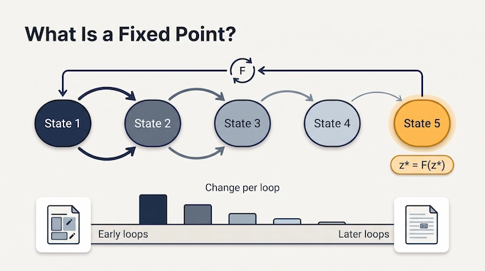
A fixed point is a state that barely changes when the recurrent block is applied again.
The compact expression is:
z* = F(z*)
Here, F is the recurrent update and z* is the settled state. A useful mental model is editing an answer repeatedly. Early revisions may change whole paragraphs. Later revisions change a word or two. Eventually another editing pass produces almost the same document.
That “almost” matters. The paper treats approximately stationary states at finite depth as fixed points for practical purposes.
The convergence is also not tidy. Different tokens can settle at different recurrence depths, and later tokens can converge before earlier ones. In the Huginn analysis, token position had only a weak relationship with convergence depth. So a fixed point LLM is not simply marching left to right until each token is “done.”
4. Why the Endpoint Can Replace Part of the Path
Suppose recurrent states evolve like this:
state 1 → state 2 → state 3 → state 4 → state 5
If state 5 is near a stable equilibrium, the model may not need every intermediate state for every operation. Part II turns that observation into four separate shortcuts.
During pretraining, gradients can be computed through only the final recurrent steps. During decoding, earlier tokens can expose only their terminal KV representation. During prefill, a student can learn to predict the endpoint rather than replaying all recurrences. During RL, saved rollout states can be reused instead of rebuilding the full trajectory before computing an update.
This is the conceptual center of the paper. The claim is not that the journey never matters. The claim is that once training makes the destination stable enough, some later computations can work from the destination directly.
5. How Terminal KV Sharing Cuts the Cache by 3×
KV-cache memory is one of the clearest wins because ordinary looped decoding can multiply cache storage with recurrence depth. If each logical visit leaves behind its own key and value banks, a model with many recurrences can carry a surprisingly large memory bill.
The tested looped transformer architecture has one prelude block, a two-block recurrent core, and one coda block. At five recurrences, that produces a logical depth of 12 block applications. With terminal KV cache sharing, however, decoding keeps one KV bank per physical attention layer, four banks rather than twelve. That is the source of the 3× smaller KV cache figure.
Does that make inference 3× cheaper? No. It makes this part of inference memory 3× smaller in this configuration. The recurrent core still runs multiple times, so inference FLOPs do not vanish with the discarded KV history.
Training also matters. Fixed-depth training performed badly when terminal sharing was forced. At 1.6B parameters, GSM8K accuracy fell from 50.6 to 21.2 under sharing. The learned-depth approach was designed to make the states tolerant of terminal context instead.
6. How Distilled Prefill Reaches 1.79× Faster
Prefill is the phase where the model processes the prompt before token-by-token generation begins. For long prompts, it can be a major latency cost.
Part II replaces repeated recurrent prefill with a smaller, non-recurrent student trained to predict the teacher’s terminal state. The teacher then performs one recurrence to construct terminal KV banks, and normal recurrent decoding continues afterward.
That shortcut works, but it is not free speed. Across the 100M, 400M, and 1.6B models, distilled prefill was about 1.5–1.8× faster on 8K prompts. The downstream average trailed the full teacher by 1.0, 2.3, and 4.5 points respectively. The gap grew with model scale. At matched latency, however, the distilled student beat simply stopping the teacher after two recurrences by 0.5–0.9 downstream points.
So 1.79× faster prefill is a real measured result, but it is a latency-quality trade. It should not be read as a free serving speedup.
7. Is Reinforcement Learning Really 2× Faster?
Yes, for a specific part of RL.
Typical recurrent RL generation first produces a rollout without gradients, then replays the model with gradients to score that rollout and compute the update. If the saved endpoint is already near a fixed point, Part II reuses it instead of replaying all recurrent steps.
With Neumann-4 updates, scoring plus backward computation was 1.99× faster on GSM8K and 2.02× faster on MBPP+ than full backpropagation through time. Performance stayed close enough to the full-BPTT baseline that the paper attributes the observed gaps partly to run-to-run variation.
But “RL is 2× faster” is too broad. In the MBPP+ experiment, rollout generation consumed 72–82% of total training time, with code verification taking another 12–15%. The reuse runs were actually slower end to end because their sampled rollouts took longer, more than canceling the update-time saving.
That caveat matters. Part II accelerates the gradient-producing update path. Whether that translates into faster wall-clock RL depends on what dominates the rest of the pipeline.
8. What Is the Learned Depth Prior?
The learned depth prior is easy to misread as adaptive inference. It is not a mechanism where the model looks at a hard question and decides, “Give me nine loops,” while using three for an easy one.
It controls where training supervision lands across recurrence depths.
A fixed training depth concentrates learning at one recurrence count and can predict well there, but the paper finds that this harms the fixed-point behavior needed for KV sharing. Huginn’s broad Poisson-log-normal prior spreads supervision across depths, which helps recurrence remain useful away from one exact depth, but it can dilute supervision around the target depth.
Part II learns a categorical distribution over training depths from prediction feedback. An entropy term prevents that distribution from collapsing too narrowly, while a budget penalty keeps the expected depth near the intended compute budget.
The distinction is important: training-depth distribution is not adaptive inference halting. The learned prior shapes the recurrent dynamics so they remain useful across depth.
9. What Is Orthogonal Input Injection?
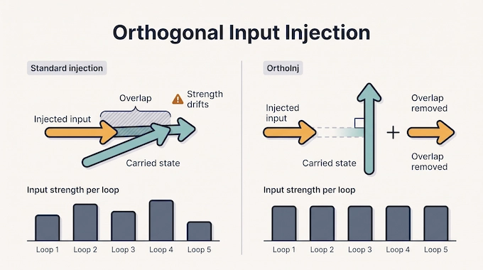
A recurrent model still needs the original input to matter after several loops. One common solution is to inject an input-derived representation at every recurrence.
The problem is that the carried state can contain a component pointing in the same direction as the injected input. Depending on its sign, that component can reinforce the new injection or partly cancel it. The effective strength of the original input therefore drifts from recurrence to recurrence.
Orthogonal input injection, or OrthoInj, removes the carried state’s component along the injected input before adding the input back. In plain English, it tries to keep each recurrence from accidentally shouting over, or muting, the fresh input signal.
Across the tested 100M to 1.6B scales, OrthoInj reduced validation perplexity by roughly 0.3–1.4% relative to the strongest injection baseline and improved the downstream average.
10. Looped Transformer vs Standard Transformer: What Do You Gain?
The useful comparison is not “small recurrent model beats big model.” It is a trade between resident capacity, logical depth, memory, and repeated compute.
A standard untied Transformer buys more depth with more unique parameters. A looped Transformer buys more logical depth by running shared weights again. That can lower parameter and KV-storage requirements, but each recurrence still consumes compute.
At 1.6B scale, the learned-prior looped model at five recurrences approached the 12-block untied baseline while using 3× fewer non-embedding parameters and 3× less KV cache. It trailed the untied 12-block model by 1.5 points on the downstream average, while substantially outperforming the four-block untied model at the same physical depth and parameter class.
That is promising, but it does not prove that a 1.6B looped LLM is generally equivalent to a much larger conventional LLM. The evidence is tied to this architecture, training setup, scale range, and evaluation suite.
A practical rule is simpler: looped models exchange additional repeated computation for lower resident parameter and memory requirements. Smaller memory footprint and lower total compute are not the same thing.
11. Does This Scale to Frontier LLMs?
This is the question the paper cannot yet answer.
The experiments span 100M, 400M, and 1.6B parameters. The authors explicitly list larger scales and other model configurations as untested, use one training seed per configuration, and say their ablations do not exhaust the design space. They also say real-world feasibility needs more study.
The evaluation appendix adds two useful cautions. Results generally use one training seed, and document-level separation between some evaluation material and the pretraining corpus was not verified. Those are not reasons to dismiss the findings. They are reasons not to promote them into a law of scaling.
There is also a systems question. A memory-saving architecture can be extremely valuable when KV cache is the bottleneck. A compute-heavy recurrent architecture may be less attractive when latency or throughput is the constraint. Frontier deployment depends on hardware, batching, context length, recurrence budget, and workload mix.
Part II gives a credible mechanism and controlled evidence. It does not yet give a production recipe for replacing today’s frontier Transformers.
12. What Part II Means for Latent Reasoning and Future LLMs
The larger idea behind latent reasoning is that model capability might scale not only through more parameters or more visible reasoning tokens, but through more internal recurrent computation.
A looped Transformer makes that third axis explicit. The same weights can revisit and refine a hidden state several times. Part II strengthens the case by showing that deeper recurrence does not always have to drag every intermediate state through every stage of the system. Near a useful fixed point, the endpoint can sometimes substitute for the path.
That is why the 3×, 1.79×, and 2× numbers matter, even after the caveats. They are not three claims that “looped models are faster.” They are evidence that fixed-point structure can remove specific depth-dependent costs: KV storage in decoding, recurrent work during prefill, and trajectory replay during RL updates.
The open question is whether those advantages survive at tens or hundreds of billions of parameters, under real serving loads, without losing the quality benefits that made the recurrence worth running in the first place.
For now, Towards Looped Models Done Right Part II does something more useful than declaring the standard Transformer obsolete. It turns fixed points from a mathematical curiosity into a practical systems idea.
If you follow recurrent architectures, test-time compute, and the next generation of language-model efficiency research, keep an eye on Binary Verse AI. We break down the papers behind the headlines, including what the benchmark numbers actually prove and what they do not.
1. What is a looped transformer?
A looped transformer repeatedly applies the same Transformer blocks across multiple recurrence steps rather than using a different set of weights at every logical layer. This allows the model to gain additional logical depth without increasing resident parameters in proportion to that depth.
2. How is a looped transformer different from a standard Transformer?
A standard Transformer normally has separately parameterized layers stacked through depth. A looped transformer reuses the same recurrent core several times, trading extra computation for lower parameter and memory requirements.
3. What is a fixed point in a looped language model?
A fixed point is a recurrent state that changes very little when the model processes it through the shared block again. Part II argues that once representations approach these states, the final state can sometimes substitute for much of the recurrent trajectory, enabling memory and computation shortcuts.
4. Are looped transformers actually faster and cheaper?
Not universally. The paper reports a 3× smaller KV cache, prefill up to 1.79× faster, and about 2× faster RL scoring/backward, but these refer to specific parts of the workflow. Extra loops still require computation, and the authors’ code-RL experiment did not become faster end-to-end because rollout generation dominated total time.
5. Will looped transformers replace today’s large language models?
There is not enough evidence to say that. The experiments currently scale only to 1.6B parameters, and the researchers explicitly state that larger models, other configurations and real-world deployment remain untested.