

How many pieces do you need to take a graph apart? A complete graph can have more than half a billion edges on 32,000 vertices, yet OpenAI’s proof shows that a constant times the vertex count always suffices. The pieces are edge disjoint cycles and single edges. The result settles the Erdős–Gallai cycle decomposition conjecture, posed in 1966. Its decisive move is to pair up vertices in sparse parts, solve smaller graphs, and use edges saved from dense parts to reconstruct the original cycles. The proof works because it saves enough vertices to pay for that reconstruction and keeps track of where every original edge goes.
Table of Contents
1. Edge-Disjoint Cycles and the Erdős–Gallai Conjecture
Theorem 1.1 of A Linear Cycle-and-Edge Decomposition of Every Graph says there is an absolute constant such that every finite simple undirected graph on vertices admits a partition of its edge set into at most parts. Each part is the edge set of a simple cycle of length at least three or consists of one edge. “Absolute” means the same constant works regardless of the graph’s density, connectivity, or degree distribution.
| Feature | What the Theorem Says |
|---|---|
| Graph | Finite, simple, and undirected, with vertices. |
| Allowed Pieces | Simple cycles of length at least three and individual edges. |
| Edge Assignment | Every edge appears once. Different pieces may share vertices. |
| New Bound | At most pieces for one universal constant . |
| Sharpness | Linear order is necessary. The optimal constant is open. |
Two cycles can pass through the same vertex. Each edge must appear in exactly one piece, so an overlapping cover can fail even if it includes every edge. Removing a duplicate edge from a cycle opens it into a path and can increase the number of pieces needed. A tree has no cycles, so each of its edges must stand alone. A tree on vertices already needs pieces.
2. How Can a Dense Graph Have Only Pieces?
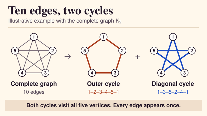
In the complete graph , label the vertices from 1 to 5. Every pair is joined, giving ten edges. Walk around the vertices in numerical order to get the first cycle. The unused edges are the five diagonals of that pentagon, and following them gives the second cycle.
| Piece | Vertex Order |
|---|---|
| Outer Pentagon | |
| Diagonal Cycle |
Read each adjacent pair as an undirected edge, including the final step back to 1. Both walks visit all five vertices and together use each of the ten edges once. This is a graph decomposition into two pieces. In bigger graphs a cycle can still use many edges at once. The difficulty is finding cycles that do this efficiently across an arbitrary graph, including regions where some edges belong to no cycle.
3. Sixty Years of Progress Toward the Linear Bound
Erdős, Goodman, and Pósa recorded the bound in 1966. Conlon, Fox, and Sudakov improved it to in 2014. Bucić and Montgomery obtained , published in 2024. Here counts how often you take a base-two logarithm before reaching at most one. It grows slowly, but the bound still leaves a multiplier that depends on .
Earlier results already gave linear bounds for some classes, including graphs of linear minimum degree. General graphs can mix regions of very different densities. Breaking them down by scale makes their edges easier to handle, but a method that spends a linear number of pieces at each scale can accumulate too much cost. The new proof charges the work across a whole prefix of scales to the vertices saved at one selected layer.
4. OpenAI’s Proof Roadmap in Five Stages
1. Split by scale. Take out long cycles and separate the remaining edges into small boxes. Inside each box, extract well-connected pieces and pass the sparse remainder to a lower scale.
2. Save edges for connections. Select one expanding layer that can pay for the prefix. Reserve some of its edges to repair cycles later. Keep enough expansion to process each piece into completed parts and a much smaller residue.
3. Route without conflicts. Use expansion to find short paths that avoid forbidden vertices. Choose the paths together so that two connections never spend the same edge and connections within one new cycle can fit together.
4. Fold and lift. Pair eligible vertices in the sparse remainder to make smaller graphs. Decompose those graphs by induction, then use reserved paths to turn the quotient cycles back into simple cycles of the original graph.
5. Balance the count. Use the saved vertices to pay for the work already done. A stronger inductive estimate covers the extra vertex counts introduced by overlapping boxes.
5. Splitting Graphs into Small Boxes and Expanding Pieces
Section 5 starts with a graph of order , meaning its number of vertices, and average degree at most . Cycles of length at least each remove enough edges that at most can be taken. Once they are gone, any subgraph larger than has a set with a small external neighborhood. Stronger neighborhood expansion would force a long cycle.
The split copies just that neighborhood into both children. Every edge is assigned to one child, so the overlap is in vertex counts only. A potential for the binary splitting process bounds the total box order by . Within a box, repeatedly cut wherever there are too few edges crossing relative to the smaller side. In a surviving piece of order , let be the set of edges crossing from to its complement. The cut expansion bound means that every satisfies
Charge each removed cut to its smaller side. A vertex can receive that charge only when its current piece shrinks by at least half. The residual box graph consequently has average degree at most for sufficiently large . It keeps the full box vertex set, and its edges enter the next scale.
6. Three Reservoirs Turn Paths Into Simple Cycles
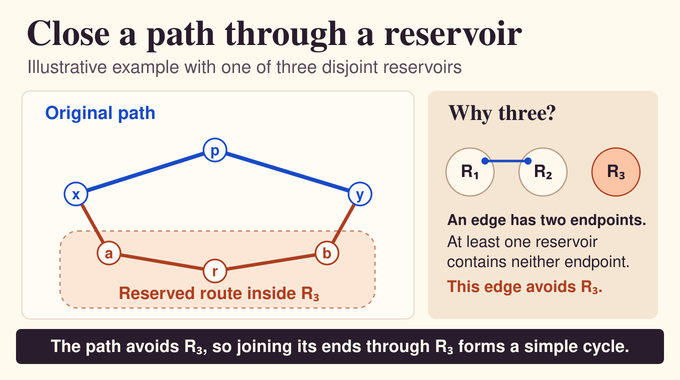
Partition the edges of a spanning expander into three expanding subgraphs. Sample three mutually disjoint small vertex sets, one in each subgraph, so that each set still supports expansion and all outside vertices have many neighbors in their respective reservoir. For each reservoir, reserve its internal expander edges and two edges from every outside vertex to distinct representatives. The choices cap the load at each representative.
Three sets suffice because an edge has only two endpoints. Every unreserved edge therefore avoids at least one reservoir and can be assigned to a complementary graph. A consequence of Lovász’s theorem partitions each complementary graph into paths with at most two endpoint occurrences per vertex. The two reserved edges at an outside vertex cover both possible occurrences.
A path closes by entering the reservoir at one representative and leaving at the other. If they coincide, the two entering and leaving edges suffice. Every added internal vertex lies outside the original path, making the cycle simple. For a piece of order , Section 4 completes at most parts, including unused access edges taken singly. The remaining edges lie inside the reservoirs, whose combined order is at most any prescribed positive fraction of once the scale cutoff is high enough.
7. Hypergraph Matching Routes Paths Without Reusing Edges
A good path for one demand can block a later demand. The expansion threshold in Lemma 3.1 makes room for all of them. With maximum route length , endpoint load , team size , and forbidden-set size , the lemma requires
Here is set by the order and expansion of the router. The proof treats each candidate path as a set of resources in a hypergraph. It claims the graph edges it uses and a token for each internal vertex paired with its team label. Disjoint choices prevent edge reuse globally. The tokens prevent two paths in the same team from using the same internal vertex, while each demand separately forbids specified vertices from its interior.
Aharoni–Haxell’s matching theorem gives one compatible choice per demand if every subfamily of demands has a union of candidates containing a matching larger than , where bounds candidate resource-set size. To establish this, the paper assumes a small maximum matching blocks a subfamily. Bounded endpoint load supplies many distinct roots, and bounded team size keeps token exclusions manageable. After deleting blocked edges and demand-specific forbidden vertices, expansion grows unions of balls around those roots. Repeatedly halving the root set and regrowing the union isolates a root whose ball reaches more than half the vertices. If both endpoint balls exceeded half the router, their intersection would give a short path using only available resources. Maximality rules that out. This contradiction supplies simultaneous routes for reservoir closures and cycle lifting.
8. Pair Folding Shrinks the Graph
After a fixed gap in scales, group the tiny descendant boxes into batches of order at most . Within a batch, pair low-degree vertices in sufficiently large intersections with a selected expanding piece. The degree cap applies to the union of all batches in the parent box. A set must have at least eligible vertices, enough to make accidental collisions rare under random pairing.
Low degree on the paired side alone is insufficient. A vertex adjacent to many members of a folding set can lose an edge each time two of its neighbors become one vertex. The proof removes edges to these heavy neighbors first. It partitions those edges into paths, takes terminal edges at heavy endpoints singly, and closes the surviving paths using reserved routes.
Each pair then becomes one quotient vertex. Edges within a pair become loops, and distinct edges between the same quotient vertices may collide. An expectation bound shows there is a pairing for which taking the loops and surplus parallel edges singly costs at most twice the total folding-set order. Each retained quotient edge keeps one original representative.
9. Cycle Lifting Reconstructs Simple Cycles
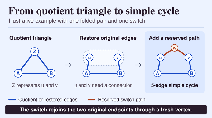
Suppose a quotient cycle arrives at a folded vertex through the representative edge ending at and leaves through the edge starting at its twin . A switch path in the reserved router joins to . If the two endpoints coincide, the representatives already join. Each original endpoint used by this quotient cycle is forbidden inside any of its switch paths.
For switches in the same router, the cycle defines a team, so their interiors are disjoint. For example, if a quotient triangle has one switch and its route is , its three representative edges plus the two route edges form a five-edge cycle. The intermediate vertex must avoid every representative endpoint. Switches in different routers of the same parent box lie in vertex-disjoint pieces. Since the quotient cycle visits distinct fibers, the original endpoints at different visits are distinct too. Together these facts make the lift a single simple cycle. A quotient singleton edge simply lifts to its original representative.
The proof bounds each vertex’s routing load across all batches by charging every demand-end occurrence to a different incident edge of the batch union. All routes use reserved edges, each at most once. A separate spanning expander remains untouched, allowing Section 4 to process what is left of each selected piece.
10. The Final Induction Gives the Linear Bound
At layer , the scale is . Write for the total order of that layer’s expanding pieces, counting pieces in different boxes separately. Section 7 finds an index where the total piece order through layer is at most a fixed multiple of . If the bound fails at a candidate index, a larger layer lies within the next 200 steps. Moving to it preserves the bound on the prefix already passed and eventually stops.
Set and . In the nonterminal case, completed work costs pieces. Quotient orders sum to at most
The remaining expander residues have total order at most . Taking the constant sufficiently large lets the net vertex savings pay for the work proportional to . Boxes can overlap, so a residual excess in the order count still needs to be paid for.
The induction uses the stronger budget , with and, for ,
Each quotient has order at most . The difference is bounded below by a positive constant times . This dominates the overlap charge of order at large scales. At the cutoff, bounded average degree makes it affordable to take the final sparse edges singly, while any small expander residues still go to induction. Since , the stronger bound implies .
11. Eulerian Graphs and Optimal Bounds
An Eulerian graph, in the paper’s convention, has even degree at every vertex and may be disconnected. Removing the cycle parts preserves even degrees. The singleton edges therefore form an even graph, which can be split into cycles using at most as many parts as there were singleton edges. This yields an Eulerian graph cycle decomposition within the same linear bound.
A vertex of maximum degree needs at least cycles to cover its incident edges, because each simple cycle contributes at most two there. Corollary 1.2 reaches this lower bound up to an arbitrarily small linear error when every cut with both sides of size at least has at least crossing edges, with and the sides and fixed. The required and minimum graph size depend on and the permitted linear error. For general cycle-and-edge partitions, certain complete bipartite graphs require pieces, where tends to zero as grows. An odd-sized smaller side forces at least one singleton at every vertex on the larger side, and the cycles have limited length. The optimal universal constant remains open.
12. Lean Verification, Scope, and Remaining Questions
OpenAI’s release attributes its results to an internal frontier model. The five stages above reconstruct the dependencies in the written proof, without assigning a chronology to the model’s discoveries. The Family 181 Lean scope note specifies the universal linear bound for finite simple graphs, including edgeless graphs. The Lean file proves the main theorem, and an independent Comparator replay reports acceptance by Lean’s kernel and the separate nanoda kernel. The replay checks the formal statement within Lean’s definitions. Corollary 1.2 and the prose arguments used to explain it belong to the manuscript’s exposition.
The proof gives an existence bound on the number of pieces. It leaves open the sharp universal constant and supplies no practical runtime benchmark for finding such a partition. Its reusable insight is that edge-disjoint cycles can survive a reduction in vertex count when the original edges and the routes that reconnect them are accounted for together. Follow Binary Verse AI for more research explainers on graph theory and machine-checked mathematics.
What is the Erdős–Gallai cycle decomposition conjecture?
It states that every finite simple undirected graph with n vertices has an edge partition into at most Cn simple cycles and single edges for one universal constant C. OpenAI’s proof establishes this linear bound.
Why are single edges necessary in a cycle decomposition?
A tree has no cycles and a tree on n vertices has n − 1 edges. For such a graph every edge must be taken as a separate piece.
Can edge-disjoint cycles share vertices?
Yes. Two cycles may pass through the same vertex, but they cannot share an edge. Each edge belongs to exactly one part of the decomposition.
How does OpenAI’s proof improve the previous result?
The previous general bound was O(n log* n). OpenAI’s proof achieves O(n) by splitting the graph at several scales, folding pairs of vertices, using reserved paths to restore cycles, and balancing these costs through a strengthened induction.
Does the proof determine the minimum number of cycles needed?
The theorem proves a universal linear upper bound for the total number of cycles and single edges. The optimal constant remains open. Certain complete bipartite graphs require at least (3/2 − o(1))n pieces, with o(1) tending to zero as n grows.
Does the result apply to Eulerian graphs?
Yes. Every finite simple graph with all degrees even has an edge partition into O(n) cycles. After removing the cycle parts from the original decomposition, the singleton edges still give an even graph, which can itself be partitioned into cycles.
Has OpenAI’s Erdős–Gallai proof been formally verified in Lean?
Yes. Family 181 formalizes the main theorem, and independent checks have reported successful kernel replay. The replay checks the formal theorem, while the manuscript presents the detailed mathematical exposition.