
Can a chemical species fade to zero even if every reaction has a directed return path? For a finite weakly reversible network governed by mass action kinetics, OpenAI’s September 25, 2026 preprint proves that it cannot, provided the reaction rates are positive constants and every species starts at a strictly positive concentration. Theorem 1.1 gives a solution for all forward time and a positive lower bound and finite upper bound for every concentration. The bounds can depend on where the trajectory starts. The result answers two questions in chemical reaction network theory with one construction. It builds a compact polytope around the initial state and uses return paths in the reaction graph to show why the trajectory stays inside.
Table of Contents
1. Can a Chemical Species Disappear in a Weakly Reversible Network?
A return path gives the system a way to rebuild a reactant complex. But the graph only records which reactions are available. It says nothing about how fast they run at a particular concentration. A step on the return path may require a species that is already scarce. Its rate could then be tiny while another reaction keeps consuming that species. To rule out extinction, the proof has to compare entire groups of reaction rates at the same state.
| Key Fact | What the Paper Proves |
|---|---|
| Network | A finite set of complexes and reactions, with a directed return path for each reaction. |
| Rates and Initial State | All rate constants are positive and every initial species concentration is strictly positive. |
| Trajectory | It exists for all forward time, stays bounded, and stays a positive distance from the boundary. |
| Geometry | Each positive starting state belongs to a compact convex forward-invariant polytope. |
| Scope of the Bound | The same bound covers all species on that trajectory and may depend on the initial state. |
The graph and the differential equation describe different spaces. The graph connects complexes, the ingredient combinations written on either side of a reaction. The differential equation moves a point whose coordinates are concentrations. The proof connects the two by ordering the complexes according to the direction in which it needs to control motion.
2. Chemical Reaction Network Theory and Mass-Action Dynamics
A network with species records a complex as a vector of nonnegative integers. With species ordered as , the complex is and is . Write for the set of complexes and for the directed reactions. A linkage class is a connected component after ignoring the arrows. In weakly reversible reaction networks, each arrow has a directed path from back to .
For a concentration vector , the source monomial is . Multiplying it by the positive rate constant gives the reaction flux. The flux scales the change vector , and summing these changes gives the mass-action equation.
Take the directed cycle with unit rates, using for its three species concentrations. Its equations are , , and . The return path for the first reaction goes through the third species. Each concentration has a production and a consumption term, while adding the equations gives zero. The sum is conserved. This simple bound comes from the particular reaction vectors, a convenience the general proof cannot assume.
3. The Boundedness and Persistence Conjectures
Boundedness of mass action systems asks whether each positive trajectory has a finite upper bound. The persistence conjecture in chemical reaction network theory asks whether concentrations along a bounded positive trajectory stay away from zero in the long run. In the paper, persistence means for every species . A coordinate could be positive at every finite time and still converge to zero. Persistence also rules out approaching zero along a sequence of late times while rising between those times.
The stoichiometric subspace is the real span of all reaction change vectors. Since is a linear combination of those vectors, motion starting at stays in the affine space . Intersecting that space with the nonnegative orthant gives the closed stoichiometric compatibility class. In the three-species cycle this is a triangle determined by the conserved sum. Other networks can have unbounded classes. Even a bounded class can touch a coordinate plane, so an upper bound leaves the boundary question open.
4. Why Earlier Approaches Could Not Establish the General Theorem
Earlier results covered different parts of the problem. Anderson proved boundedness for one linkage class. Craciun, Nazarov, and Pantea obtained boundedness and permanence for weakly reversible systems with two species. Pantea proved persistence of bounded weakly reversible trajectories with two-dimensional stoichiometry, which can involve more than two species. Craciun’s revised toric differential inclusion manuscript gives persistence for bounded positive trajectories with uniformly positive, bounded variable rates. The September 25 proof supplies both bounds for constant rates across arbitrary finite networks satisfying weak reversibility.
The preprint also identifies a gap in the 2010 argument of August and Barahona. A large product of concentrations does not ensure that the monomial with the larger sum of exponents dominates. Consider with both rates equal to one. At the states with , the product grows without bound as grows. Yet the source monomial is smaller than , even though its total degree is higher.
The family of states refutes the monomial inference. Each trajectory still conserves , so its two concentrations stay bounded. The new argument compares individual source monomials in the directions that matter for confinement.
5. OpenAI’s Theorem on Global Boundedness and Species Persistence
Theorem 1.1 applies to finite weakly reversible mass action systems in every species dimension . With positive constant reaction rates and , the solution exists for all . There is a single , depending on the network, the rates, and , such that
The statement includes multiple linkage classes, isolated complexes, and empty reaction sets. An unbounded compatibility class is also allowed. For instance, the reversible one-species network spans the whole concentration axis. With unit rates its equation is , which drives a positive state toward one. The theorem generalizes confinement beyond this scalar sign argument.
In particular, any sequence of times tending to infinity has a subsequence along which the concentrations approach a point inside the positive box. The entire set of such limit points is separated from the boundary. That is the dynamical content of persistence in chemical reaction networks.
6. The Geometric Transformation From Concentrations to Exponents
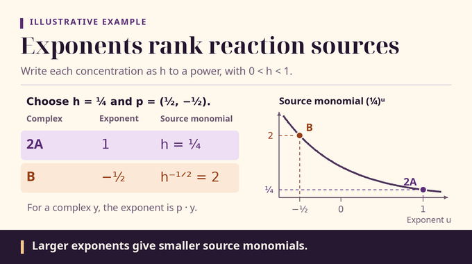
Choose a scale and write . Let denote the resulting concentration vector. The exponent cube maps onto the concentration box . A negative exponent corresponds to a concentration above one. A positive exponent corresponds to one below one. At fixed , the exponent is , so making small moves the exponent of that concentration toward zero.
For complexes and , a larger dot product therefore gives a smaller monomial. If two source exponents are separated by a fixed positive gap, their monomial ratio can be made arbitrarily small by shrinking . For example, assigns exponents and to and , respectively. Their monomials are and . The proof uses these comparisons to control motion in concentration space, where the trapping set will have flat faces.
7. Affine Labels That Preserve Critical Comparisons
A label pairs a fixed slope with an offset . The paper takes the lower envelope over the finite family , giving a concave, piecewise-affine function.
A label is active at when its affine value attains that minimum. Lemma 2.1 constructs the family for any prescribed positive slope-dependent tolerance . Corollary 2.2 makes the guarantee uniform across the exponent cube for sufficiently small .
The infinity norm is the largest coordinate error. The construction starts by fixing the smallest exponent, which controls the largest concentration. It uses induction on selected coordinates with larger exponents. Negative offset terms make certain raised slopes competitive when the concentrations on those coordinates are small enough. Compactness extends the local guarantees to neighborhoods of the smallest exponent. Shifting each selected family by a common offset then makes a minimizing label come from a suitable neighborhood. Adjacent neighborhoods overlap at the cuts, so either family is admissible at a tie.
The tolerance can shrink near a hyperplane where a slope comparison vanishes, while remaining positive on that hyperplane. The proof applies this to coordinate directions and differences of every pair of complexes. Each strict active-slope comparison then has the same sign in exponent space and a gap of at least . Exact ties in slope can group unequal monomials. The finite slope family fixes before the final choice of .
8. Directed Reaction Paths and the Flux-Domination Lemma
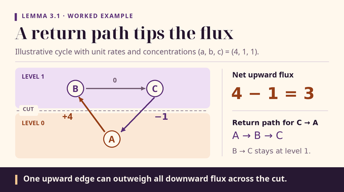
Lemma 3.1 orders complexes by the level of an active slope. Put a cut between two consecutive distinct levels. If an edge crosses downward, its return path has to cross upward somewhere. The source of that upward edge lies below the cut. Every downward edge starts above it, so its source monomial is at most times the chosen upward source monomial. With sufficiently small, times the sum of all rate constants is less than the smallest rate constant. One upward edge then outweighs the entire downward flux across that cut.
In the unit-rate cycle from Section 2, assign levels zero to and one to and . For the illustrative state , the directed return path for the downward edge includes the upward edge. The largest downward-to-upward source ratio is , and multiplying it by the sum of the three unit rate constants gives .
| Reaction | Role at the Cut | Contribution to Net Upward Flux |
|---|---|---|
| Upward crossing | ||
| Both ends at level one | ||
| Downward crossing |
The cut has a unit gap and contributes three to the directional derivative. In the general proof, let be the distinct levels and the upward flux minus the downward flux across the cut after level . A reaction crossing several cuts contributes its flux at each cut, weighted by the gap and signed by the crossing direction. Summing gives
The all-pairs comparison lets one upward edge outweigh downward flux from another linkage class. When there is only one level, the sum is empty and the derivative in that direction is zero.
9. Why Every Active Branch Must Point Inward
Write for the finite affine minimum. At a point where several labels tie, an infinitesimal forward step picks out the branch with the smallest first-order change. Inactive branches have a positive gap at the current point and cannot close it instantly. If is the set of active labels, Lemma 3.2 gives the right derivative along the solution.
For a simple illustration, take the minimum of and . At , both branches are active, and the right derivative is even though one branch increases. In the reaction network, the flux estimate checks every tied branch, making the minimum derivative nonnegative. The paper turns that one-sided derivative statement into monotonicity by adding a small positive linear function of time, then letting its slope tend to zero. Thus is nondecreasing along any trajectory segment inside the box.
10. The Invariant Convex Polytope That Completes the Proof
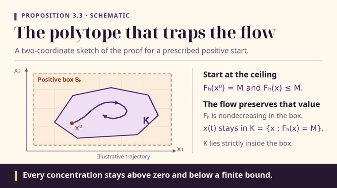
At the prescribed , sufficiently small makes each initial exponent smaller than in absolute value. The coordinate sign constraints force every active slope there to be zero. One such label supplies a constant branch with value . Since is the minimum over all branches, this constant is a ceiling everywhere. The maximum set is
At the box boundary some exponent has absolute value one. The constant branch cannot be active there because its tolerance is . Thus misses the boundary. Its half-space description makes it closed and convex. A line segment from to any point of outside the box interior would cross the boundary inside . Therefore the whole set lies inside the box and is compact.
Start a solution anywhere in . Until a first contact with the box boundary, monotonicity and the ceiling force to stay at . This also holds at the putative first contact, contradicting the boundary exclusion. The trajectory stays in . The polynomial vector field is bounded there, so a finite maximal forward time would give a limiting state in from which the solution could continue. This proves global existence and yields the concentration bounds with .
11. What the Proof Establishes and Where Its Scope Ends
The invariant polytope can meet several compatibility classes. Its intersection with the class of is compact, convex, and forward invariant. Corollary 3.4 uses Brouwer’s theorem to find fixed points of flow maps for successively shorter positive times. The mean velocity over each short return is zero. As the return time shrinks, the vector field at a limit of those points must vanish. This recovers Boros’s existence result for a positive equilibrium in each positive class.
Convergence requires further reasoning. Under complex balance, there is a positive state where incoming and outgoing flux agree at each complex. In that case the Horn–Jackson entropy decreases along trajectories, with zero derivative only at equilibria. Compact confinement and LaSalle’s invariance principle give convergence to the unique positive equilibrium in the class. Classwise permanence would instead require one common compact positive region that eventually contains every positive trajectory of a fixed class. The September 25 manuscript gives bounds for each initial state. A separate October 5 preprint treats the stronger permanence result for fixed positive rates, with a common absorbing set for each positive compatibility class.
OpenAI’s Lean scope note lists global forward existence and a common lower and upper bound for all species and all global forward solutions from a prescribed positive state. The Lean implementation also proves the invariant-polytope proposition. The formal statement allows the bound to depend on that state, the network, and the rates. The scope note specifies the September trajectory theorem even though its heading uses the broader family title. The theorem gives a qualitative guarantee for the deterministic model. Estimating the smallest concentration or the time to approach equilibrium in a specific system requires further analysis.
The advance for chemical reaction network theory is a way to turn directed return paths into confinement of the full concentration trajectory, even when conservation laws leave its class unbounded. Follow Binary Verse AI for more research explainers on dynamical systems, directed graphs, convex geometry, and Lean-checked proofs.
What does weak reversibility mean in a chemical reaction network?
A reaction network is weakly reversible if every directed reaction has a directed path leading back to its starting complex. The return path can pass through intermediate complexes. This graph property is central to the boundedness and persistence theorem.
Can a chemical species disappear in a weakly reversible mass-action system?
The theorem gives a positive lower bound for every species at all future times in a finite weakly reversible mass-action network with positive constant reaction rates and strictly positive initial concentrations. No concentration can approach zero, even along a sequence of increasingly late times.
Why was the persistence conjecture difficult to prove?
Earlier methods established persistence or boundedness under additional restrictions, such as a single linkage class, two species, or a bound on the trajectory. A 2010 paper stated the general result, but its proof contained an unjustified inference about which reaction monomial dominates. The September 2026 proof handles arbitrary finite weakly reversible networks with positive constant rates through a geometric construction.
How does OpenAI’s proof establish boundedness and persistence?
The proof constructs a concave, piecewise-affine function whose active slopes preserve critical comparisons between reaction monomials. Weak reversibility then guarantees nonnegative net upward flux across cuts between ordered levels of the reaction graph. These estimates yield a compact, convex, forward-invariant polytope that traps each positive trajectory away from zero and infinity.
What is the difference between persistence and permanence?
Persistence means that concentrations along an individual positive trajectory remain asymptotically bounded away from zero. Permanence requires a common compact positive region that eventually contains every positive trajectory in a fixed compatibility class. The September 25, 2026 paper proves trajectory-level boundedness and persistence. The October 5 follow-up proves classwise permanence for fixed positive rates.
Does weak reversibility guarantee convergence to equilibrium?
The paper proves convergence under the additional assumption of complex balance. A Lyapunov function and LaSalle’s invariance principle give convergence to the unique positive equilibrium in each class in that case. For general weakly reversible systems under the theorem’s assumptions, the paper recovers the existence of a positive equilibrium in every positive stoichiometric compatibility class.
Has OpenAI’s persistence proof been formalized in Lean?
Yes. OpenAI’s Lean formalization covers global forward existence and boundedness and persistence for finite weakly reversible mass-action systems with positive constant rates and positive initial conditions. The bound may depend on the network, rates, and initial state. The published scope note covers the September trajectory theorem.