

Pick 1, 3, 6 and 8. You can subtract the smaller number from the larger in any pair without getting a perfect square. Try adding 5 and the construction breaks immediately, since 5 and 1 differ by 4. How large can square difference free sets get when you can choose from all the integers up to ? OpenAI’s preprint proves that their size is at most for absolute constants and . The exponent stays below 1 by a fixed amount, so the largest possible share of the interval falls at least as fast as a fixed power of .
Table of Contents
1. How Many Numbers Can You Choose Without a Perfect-Square Difference?
A square-difference-free set excludes every positive perfect square from its pairwise differences. In , the six positive differences are . The forbidden differences begin . A set can contain square numbers, including 1, as long as the distances between its members satisfy the rule.
| Item | Key Fact |
|---|---|
| Universe | The integers from 1 through . |
| Forbidden differences | Positive perfect squares such as 1, 4, 9 and 16. |
| Extremal quantity | The largest possible set size, denoted by . |
| New upper bound | for absolute constants and . |
| Remaining question | The optimal growth rate of . |
There is also a graph interpretation. Make each integer a vertex and join two vertices when their distance is a perfect square. A legal choice is an independent set, meaning it contains no edge. As the interval grows, so does the list of forbidden distances. This is why a small example can illustrate the rule but says little about the long-run maximum.
2. OpenAI’s Proof and the First Fixed Power Saving for Square Difference Free Sets
Write and let be the maximum cardinality of a square-difference-free subset of . Theorem 1.1 of the September 24, 2026 manuscript proves that for every integer ,
The constants are absolute, meaning they depend on neither the interval length nor the choice of set. The constant makes the estimate uniform even at small lengths. The saving is the fixed positive in the exponent. Doubling the length, for example, multiplies the upper bound on the allowable density by . Finding the exact maximum is a separate problem.
3. The Furstenberg–Sárközy Theorem and the Previous Mathematical Limit
Furstenberg and Sárközy independently answered a question of Lovász. They proved that an infinite set of positive integers with positive upper density must contain two elements a positive square apart. Here upper density is the limit superior of the proportion of integers selected in . The finite formulation is , meaning the maximum density tends to zero. Furstenberg’s proof used ergodic theory, and Sárközy’s used the circle method. Sárközy gave a logarithmic saving. Pintz, Steiger and Szemerédi sharpened it, and Bloom and Maynard improved it further by controlling additive relations among rational frequencies.
Green and Sawhney’s bound had the form , for an absolute , up to a constant multiplier. Their arithmetic level inequality controlled rational Fourier coefficients within a density-increment argument. A separate October preprint by Steve Fan and Andrew Lott strengthened that rate to , with . Both savings are stretched exponential in the logarithm of the interval length. The fixed power saves more asymptotically because eventually exceeds either square-root expression in the exponent.
4. The New Proof Strategy and the Quantity That Contracts
The proof replaces the indicator , which equals 1 on the chosen set and 0 elsewhere, with a real Fourier lift . This lift describes how the set is distributed across residue coordinates for a collection of primes. Its constant Fourier coefficient is the original density, even though the lift can take negative values. The proof then samples a correlated tuple of residue vectors with a fixed, even number of slots. It defines
The expectation is over the full tuple law. The sampled values are correlated, so their product cannot be averaged by multiplying their individual means. A seminorm bound for the law gives
Polynomial decay for then bounds the density after taking a th root. One estimate compares with its counterpart on shorter intervals. Another makes some of the terms in that comparison small enough to force a strict contraction.
5. Finite-Field Square Constraints and Why They Mix
For an odd prime , the field consists of the residues modulo . Its nonzero squares are the values for nonzero residues . Exactly half the nonzero residues are squares, since each has two roots. Modulo 7, the nonzero squares are . An ordered edge from to passes the test when belongs to that list. Thus the edge from 1 to 3 passes, while its reverse has difference 5 modulo 7 and fails.
The finite-field estimate explains how these tests behave in combination. On the Fourier characters of the field, the operator for a single edge test after subtracting has norm at most . The nonconstant eigenvalues are controlled by a quadratic Gauss sum of magnitude . For a fixed directed graph with edges, no loops and at most one edge per unordered vertex pair, the probability that independent uniform labels pass all tests differs from by at most . A separate four-copy argument gives an operator mixing bound of order for the constraints between two lists of labels.
6. Reflection-Positive Probability Laws and the 24-Cycle
Section 3 constructs one tuple law for each sufficiently large prime. The 24 slots on the designated directed cycle sit inside a much larger index set of permutation words. Swapping two symbols in one word block pairs up all slots and cuts the index set into two halves. Reflection positivity says that the matrix coupling the two half-tuples is symmetric positive semidefinite. In particular, averaging the product of the same real function on the two reflected halves gives a nonnegative value, even when that function changes sign.
To achieve this, the construction mixes measures indexed by marked blocks. Marking a block provides a positive form strong enough to dominate the small negative part at its corresponding cut. In the full probability law, the exceptional submeasure has mass at most . After removing that part and normalizing, every edge of the designated cycle has a nonzero square difference, and each ordered edge pair is uniform among all pairs satisfying that constraint. Both laws provide conditional mixing for a single label given all the others. The proof uses reflection positivity for the full law and the exact edge distribution for the normalized nonexceptional law. Each prime’s tuple is sampled independently of the other primes’ tuples. The dependence that matters is between slots within a prime, which lets the law favor particular modular differences.
7. Signed Fourier Lifts, Multilinear Seminorms, and Conductor Decay
The lift retains the rational Fourier coefficients of whose reduced denominators are squarefree and at most , with . The prime factors must come from the selected large primes. The reduced denominator, called the conductor, is the product of the primes at which the character is nonconstant. The zero frequency has conductor 1. Cutting off the denominators can remove a joint oscillation while keeping its separate prime components, so even an indicator function can give a negative lift.
Repeated Cauchy–Schwarz across reflection cuts bounds the absolute value of a mixed tuple average by a product of the seminorms of its individual real inputs. Each seminorm is the th root of the average with the same input in every slot. This gives the triangle inequality and, through translation symmetry, the bound on the mean. Conditional mixing supplies a different estimate. If one slot has only conductors above , tensoring the single-prime bounds gains a factor in the mixed estimate, relative to the relevant moment norms. The manuscript bounds every fixed moment of the lift by for bounded inputs on the interval lengths used in the proof, even after retaining arbitrary collections of complete denominator classes. These bounds let the conductor gain dominate truncation errors. Fixing some residue coordinates incurs an additional, controlled cost.
8. The Signed Kernel That Detects Actual Integer Square Differences
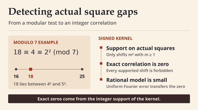
Passing a modular test does not settle the integer question. The integer 18 is a nonzero square modulo 7 because it reduces to 4, yet 18 lies between consecutive integer squares. Section 6 builds a signed kernel whose support consists entirely of positive integer shifts . Its weights restrict roots to a congruence class and use an alternating sum over squarefree divisors. At a retained rational frequency, the divisor terms combine to give the quadratic average over units, the residues coprime to the denominator. A uniform unit modulo a prime has a uniformly distributed nonzero square, matching the cycle-edge law.
The kernel’s Fourier transform approximates that of a rational-frequency model uniformly, with error at the kernel cutoff . For two functions supported on selected residue classes and on ordered portions of , the correlation with the actual-square kernel vanishes because each shift in the kernel’s support would require a forbidden pair. The uniform transform estimate transfers that zero to a small bound for the rational model. The signed weights can therefore do the Fourier matching without weakening the exact arithmetic cancellation.
9. Square-Step Progressions and Why Rescaling Preserves Avoidance
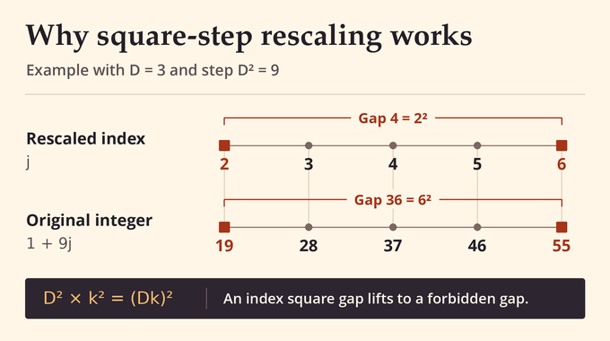
Fixing a group of prime coordinates of sufficiently small product, together with the small-prime modulus, pins down a residue class modulo an integer . The proof splits the class into progressions with step . For example, positions 2 and 6 in the progression have index difference 4, so their original difference is 36. In general, an index difference lifts to . Every rescaled subset therefore still avoids square differences. The choice of step matters. With step 3, a difference of 4 in the indices would lift to 12, which is allowed in the original set. A residue class modulo 3 must therefore be split into three classes modulo 9 before this rescaling argument can be applied.
Each rescaled set fits in an interval of length . On the remaining prime coordinates, multiplication by and translation preserve the tuple law. Using this symmetry, the mixed seminorm inequality and a conductor cutoff, Proposition 7.2 controls the specialized functional by the maximum at length , with a multiplicative factor approaching one and a power-decaying additive error. The comparison holds for every residue specification, even when different slots are assigned different residues.
10. Ordered-Interval Contraction and the Edge That Forces Cancellation
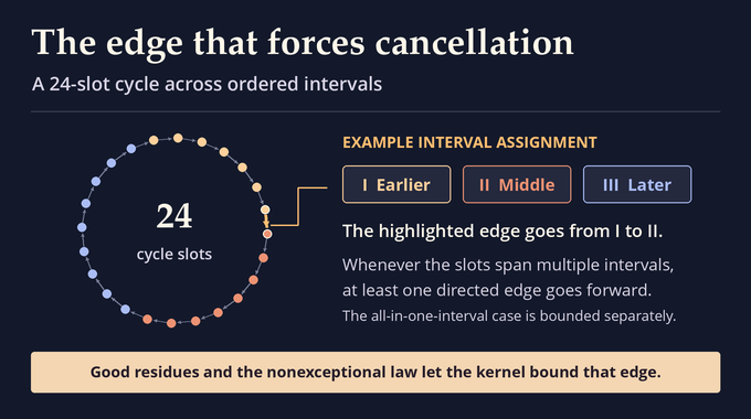
The proof uses a fixed modulus containing 8 and every odd prime below the tuple-law threshold. A residue assignment is good when every directed cycle edge has difference 1 modulo 8 and a nonzero square modulo each of those odd primes. A 24-step loop can close at all these moduli. Modulo 8, use 24 increments of 1. At each odd prime there is a pair or a triple of nonzero squares summing to zero, so the paper repeats that pattern. The Chinese remainder theorem combines the increments. The resulting proportion of good assignments is fixed and positive. The proof needs only one valid sequence of increments to get a lower bound on that proportion. The starting residue can vary freely, as can the residues at every slot off the cycle.
Now split into many consecutive intervals and expand each slot by its interval choice. The chance that all 24 cycle slots land in the same interval is small, and the moment bounds keep that contribution small. In every other assignment some directed edge goes from an earlier interval to a later one, since a cyclic sequence with no increase must be constant. Truncate and expand the other slots, then use the selected edge’s square-pair law on the remaining coordinates. The ordered kernel estimate now applies. For good residue assignments, the entire nonexceptional contribution is bounded by a negative power of .
11. Exceptional Terms and the Final Power-Saving Induction
Let be the maximum of over square-difference-free sets in . For a subset of the large primes in the lift, write for their product and for the product of their exceptional masses. Inclusion–exclusion expands the product of the prime measures so each term involving exceptional measures is weighted by . Moment estimates handle large . For small , the progression comparison sends the problem to . The empty subset gives the scale .
The resulting recurrence weights the ordinary shorter-scale bound by . On the good fraction , only exceptional terms and power-decaying errors remain. A trial bound costs a factor when inserted at a shorter scale. Since every exceptional prime contributes at most , the sum of over nonempty is at most for the paper’s parameter choices. Choosing sufficiently small ensures
That margin absorbs the scale-comparison factor and the additive error for large . Strong induction gives , and taking the th root of the density inequality gives .
12. What OpenAI’s Proof Settles and What Remains Open
The power saving answers Green and Sawhney’s fixed-exponent question. The proof’s constants reflect the size of the finite construction and the small guaranteed proportion of good assignments. The manuscript calls the saving extremely small and supplies no useful numerical value for it. A lower-bound construction by Dmitry Krachun, cited in the paper, achieves a growth exponent above . The optimal growth exponent remains open.
The theorem also gives a polynomial bound for the square-difference coloring problem. In an -coloring of , the largest color class has at least elements. If , this exceeds the bound for any square-difference-free set, forcing two integers of the same color a square apart. Only the endpoints need that color. In the graph from Section 1, write for the square-difference graph and for its chromatic number, the least number of colors needed to give adjacent vertices different colors. The same argument yields
OpenAI announced its mathematics release on October 6, 2026. Its Family 182 Lean documentation identifies the formalized statement as the uniform fixed-power-saving bound for square differences, for every . The comparator specifies the target theorem, and the release identifies a separate solution module. Independent human review of the manuscript is a separate question.
For square difference free sets, the new bound shows what becomes possible when exact arithmetic cancellation and uniform comparison across scales work together. Follow Binary Verse AI’s coverage of AI-generated mathematical proofs, including the Erdős–Turán conjecture, where the extremal question concerns sums and their representations.
What is a square-difference-free set?
A square-difference-free set contains no two distinct integers whose absolute difference is a positive perfect square. For example, is square-difference-free because none of its pairwise differences equals .
How many numbers can you choose without two differing by a perfect square?
For integers between 1 and , OpenAI’s proof establishes that every square-difference-free set has at most elements, where and are absolute constants. This bound limits the largest possible set size for every .
What is the Furstenberg–Sárközy theorem?
The Furstenberg–Sárközy theorem establishes that a set of positive integers with positive upper density must contain two elements differing by a positive perfect square. Equivalently, the maximum size of a square-difference-free subset of satisfies .
What is a fixed power saving, and why does it improve the earlier bound?
A fixed power saving bounds the maximum density by for some constant . Green and Sawhney’s earlier bound on the set size had the form , up to a constant factor. A fixed power of gives a faster asymptotic decay in density.
How does OpenAI’s proof establish the power saving?
The proof constructs reflection-positive probability laws over finite fields, applies signed multilinear inequalities to Fourier lifts, and builds a kernel supported on actual integer square differences. Rescaling, interval cancellation, and a weighted induction give polynomial decay for a quantity that controls the density.
Does OpenAI’s proof determine the optimal exponent or the exact maximum set size?
Both remain open. The proof establishes that an absolute positive saving exponent exists, but the exponent obtained is extremely small and the manuscript supplies no useful numerical value for it.
Has OpenAI’s square-difference-free proof been formalized in Lean?
Yes. OpenAI’s Family 182 documentation identifies the main fixed-power-saving theorem as the formalized result and points to its comparator statement. This scope concerns the uniform square-difference bound for every . Independent human review of the 48-page manuscript is a separate question.