
A round disk can survive every stage of a conformal approximation and still fail to fill its hole in the limit. That gap is the central difficulty of the Koebe circle domain conjecture. In a manuscript dated September 23, 2026, OpenAI proves that every domain on the Riemann sphere has a conformally equivalent model whose complementary components are round disks or single points.
The proof handles even uncountably many components. Its strategy is to choose analytic tests before taking the limit, then carry those tests through finite approximations. Small real-valued tests force unmarked components to shrink to points. At a marked component, the proof rules out any excess beyond its limiting disk.
Table of Contents
1. What Is the Koebe Circle Domain Conjecture?
The Riemann sphere, , is the complex plane with one point at infinity. A domain is a nonempty connected open set. Two domains are conformally equivalent if a holomorphic bijection with a holomorphic inverse takes one onto the other. In local coordinates this map preserves angles, while distances and areas can change. A circle domain is one whose complementary connected components are closed round disks or singletons. Roundness is understood on the sphere, so the closure of the exterior of an ordinary Euclidean circle also counts as a round disk.
In Theorem 1.1 of the September 2026 manuscript, is the given domain, is a circle domain, and is the conformal equivalence. The circle domain uniformization theorem can be written as follows.
| Topic | What the Paper Establishes |
|---|---|
| Manuscript | OpenAI preprint dated September 23, 2026. |
| Theorem 1.1 | Every domain on the Riemann sphere has a conformal circle-domain model. |
| Hole Shapes | Closed round disks and singletons, with no bound on the total number of components. |
| 1993 Result | He and Schramm covered countably many complementary components in 1993. |
| Proof Mechanism | Transfer compatible tests to finite circle domains, then use their estimates to control all limiting components. |
The annulus already has the required form. Its complementary components are the closed unit disk and the closed exterior of the circle of radius two, including infinity. A punctured unit disk instead has a singleton at the origin and a closed round exterior. A Cantor set on a line gives a less familiar example. Its sphere complement is connected, and each removed point is its own component. The upper and lower half-planes connect through the gaps in the set. This circle domain has uncountably many point holes.
2. Why the General Conjecture Remained Unsolved for Over a Century
Koebe posed the problem in 1908 and proved the finitely connected case. He and Schramm’s 1993 theorem extended it to domains with at most countably many complementary components. Schramm subsequently developed transboundary extremal length and used it for further uniformization results, including domains bounded by points and uniformly controlled quasicircles. Later work covered domains satisfying geometric hypotheses, including spherical Gromov-hyperbolic domains and certain domains with quantitative control of their complementary components.
For uncountably connected planar domains, an enumeration of all components is unavailable. The boundary can also lack the geometry required by those partial results. OpenAI’s argument marks only a countable subset. The topology and estimates still account for the full collection of components, including every label outside that set.
3. Why Finite Circle-Domain Approximations Were Not Enough
An interior exhaustion fills the domain with an increasing sequence of simpler subdomains. Finite circle-domain approximations then come from uniformizing those finite stages. The maps can converge on every compact subset of the original domain even as the shapes of the image holes remain hard to identify. Local uniform convergence provides information on fixed interior curves. Boundary components are recovered by intersecting the regions bounded by whole sequences of those curves.
Following one distinguished disk through the finite models gives a round subset of the corresponding complementary component. That component could still have extra material, such as an attached arc. A component without a distinguished disk has even less shape information at this stage. Rajala’s work on uniformization by exhaustion gives a countably connected example in which the maps along an interior exhaustion converge to a map with a noncircular complementary component. The Koebe conjecture proof therefore imposes controls on the finite stages before applying compactness.
4. The Quotient Sphere: Turning Complicated Holes Into Points
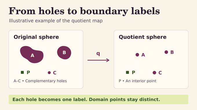
The proof collapses each complementary component to one point by a quotient map . Every point of the domain stays separate. Each complementary component is a nonseparating continuum, meaning a compact connected set whose removal leaves a connected sphere complement. Together with the closed decomposition relation, this lets Moore’s theorem identify as a topological sphere. The boundary-label space is compact and totally disconnected. The paper calls it the dust.
Finite families of disjoint disks in the quotient cover the dust, with smooth boundaries lying in the original domain. The proof refines these covers so their maximum quotient diameter tends to zero. Their exteriors give nested compact cores that eventually contain every compact subset of the domain. For a label , the nested surrounding curves isolate that end. The quotient supplies the topology for approaching it, and the original conformal structure supplies the measurements on the domain.
5. Compatible Coordinates and Dirichlet Energy
A coordinate is either a bounded smooth real function or a locally real function on the lifted domain portion of a punctured quotient disk. In the latter case, one positive circuit around the selected label adds one. Its differential is single-valued and has finite Dirichlet energy. For a real coordinate on , with denoting spherical area, the energy is
At a nonsingular boundary label , the range between the lower and upper limiting values is bounded by a budget . These budgets are square-summable in , with sums defined as suprema over finite subsets. Only countably many labels can have a positive budget. Outside a countable set of flagged labels, each coordinate defined there has a unique limiting value, taken modulo one for a periodic coordinate.
The level sets include both domain points and the boundary labels whose limiting ranges contain the chosen level modulo one. A periodic coordinate’s singular label belongs to every level. For almost every choice of levels, a finite union of earlier level sets has finite length inside the domain and only countably many nontrivial connected components. Compatibility, condition (P), requires that for almost every tuple of levels, a new level avoids free boundary labels on any nontrivial component of that earlier union.
6. Finite Transfer: Preserving Conformal Structure While Controlling Energy
Theorem 3.1 transfers a finite ordered list of compatible coordinates to a finite bordered completion. It keeps the spherical metric and all selected coordinate values on a neighborhood of the retained core, within each coordinate’s region of definition. Outside the core it permits a new conformal structure. For tolerance , the sum of the transferred energies outside the core is less than . For each test, the excess of nonsingular terminal boundary oscillations over the original budgets has norm less than . The designated terminal hole retains period one for its periodic test, and other holes in that test’s region have period zero.
To build the completion, the proof uses randomly shifted staircases whose transitions lie near sampled levels. Small tail energies bound the integrals of the pairwise wedge products by Cauchy–Schwarz. Compatibility lets the construction cap regions where at most one staircase varies on the surrounding collar. The extensions there have differentials of rank at most one. A metric adapted to these differentials keeps the tail energy small, while a finite set of terminal disks is left excised. Classical finite uniformization then produces circular holes in the new structure.
7. Normalized Limits and the Problem of Boundary Protrusions
A Möbius change puts infinity in the source domain, and all completions retain a common exterior region. The finite maps are normalized at infinity by . An exterior area estimate bounds their complementary disks, and compactness gives a subsequence converging locally uniformly to an injective conformal map on the original domain. Every compact subset eventually lies in the unchanged structure. Along the same subsequence, the distinguished disks for all countably many marks converge, allowing a limiting radius of zero.
Nested images of the surrounding curves identify one complementary component for each label. The distinguished disk at a mark stays on the bounded side of every fixed surrounding curve in the limit. Lemma 3.3 therefore gives
This inclusion still permits a protrusion, and there is no distinguished disk to use at an unmarked label.
8. Tagged Paths, Energy Barriers, and Probability Laws
The argument adapts transboundary extremal length. A path can visit the dust in the quotient, so its cost adds a boundary toll to the weighted arclength spent inside the domain. The toll is charged at every visit time, including repeat visits, with endpoint tolls omitted in the relevant tests. Tags identify portions that follow earlier level unions. Bounds on the remaining contacts let the proof cut and concatenate paths along collars while controlling interactions with prior levels and previously selected path laws.
A real barrier takes value zero on an interior testing set and one on a surrounding curve at the target end. Its controlled size combines the gradient’s norm with the boundary budget’s norm, with a localized version for paths subject to gates. If a sufficiently small compatible barrier is unavailable, the path family has positive modulus. Modulus–probability duality converts that lower bound into a probability law with square-integrable mean arclength density.
A fusion argument combines information from countable boundary tests and atomless measures. A hit probability counts a label once per sampled path, even when a path revisits it. Theorem 5.1 yields a single law with square-summable hit probabilities on all of and separate bounds on expected visit counts at prescribed countable sets.
9. Why Unmarked Components Must Collapse to Points
If uncountably many ends lacked a small barrier at a fixed tolerance, each would admit a path law. The proof finds a shared surrounding disk and four boundary arcs in cyclic order. Two independent paths to one end, entering through the first and third arcs, connect those arcs through that end. Two paths to a different end can connect the second and fourth arcs. Alternation forces a crossing. The event has probability bounded below, while the localized arclength and dust-hit estimates make every cross-pair intersection too unlikely. The exceptional ends are therefore countable. A countable basis lets the authors select compatible barriers at arbitrarily small tolerances covering every end outside a countable marked set.
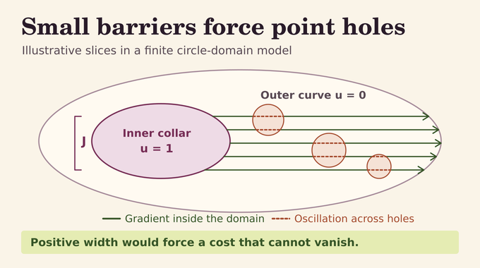
Now suppose an unmarked limiting component has a projection containing an interval of positive length. Parallel segments in the finite models must cross from a collar where a transferred barrier is one to an outer curve where it is zero. On each segment, that unit change is paid for by the integrated gradient and by oscillations across crossed holes.
For example, a disk of radius and oscillation bound contributes at most after integrating over the lines, since the lines meeting it occupy a transverse interval of length . Disjoint disk interiors bound the sum of squared radii, so Cauchy–Schwarz controls the total payment. In Theorem 6.5, each selected barrier survives every sufficiently late finite transfer. After passing to the limit for that fixed barrier, write for the width of the chosen interval and for a uniform target radius. The line estimate gives
The left side is fixed as the norms on the right tend to zero. The contradiction forces the component to be a singleton.
10. How Period-One Tests Eliminate Every Remaining Protrusion
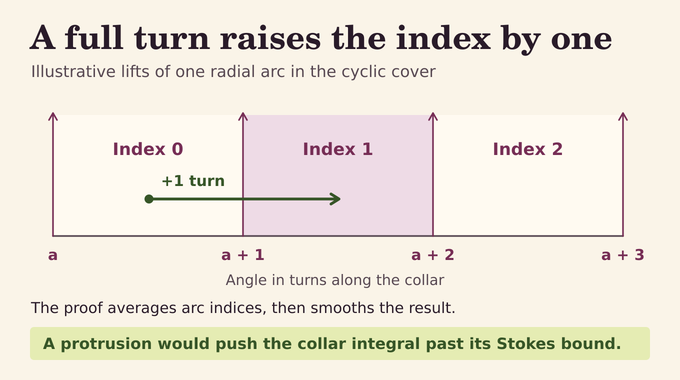
For a proposed protrusion at a marked end, Lemma 7.4 first looks for a small compatible real barrier in a localized region. When it exists, the parallel-line estimate excludes the protrusion. Otherwise, a gated path law produces a compact family of simple arcs from a deep collar to the end. In the cyclic cover, integer translates of each lifted arc divide the cover into successive regions. The index of a point increases by one under a full turn. For a straight radial arc in a punctured disk, use an angular lift measured in turns, with starting angle . The translated rays sit at for integers . Off the rays, the index is , which increases by one when increases by one. Averaging the indices of the actual arcs, then smoothing, gives a period-one test with small energy and small boundary oscillations at the nonsingular ends.
The boundary differential of the unsmoothed average records the distribution of arc starts on the collar. The gates keep those starts a positive distance from the distinguished disk in the proposed limit. Consequently, integrating distance to that disk against the test differential along the image collar gives a positive lower bound that persists after smoothing. In the finite models Stokes’ theorem bounds the same integral by the small energy and the oscillations at the other holes. The marked hole’s own term vanishes as an offset circle approaches it, since the distance tends to zero there and the period is one. The incompatible bounds exclude a neighborhood of the proposed map and disk. A countable basis of such pair spaces allows all bad pairs to be covered using countably many tests.
11. Completing OpenAI’s Proof: What the Circle-Domain Theorem Establishes
Theorem 7.5 keeps any prescribed countable compatible list and mandatory marks, then appends both kinds of tests as needed. The final diagonal transfer eventually includes each fixed test and mark while the cores exhaust the domain and the errors tend to zero. Every resulting normalized diagonal limit has singleton components at unmarked ends and exactly the distinguished disks, possibly singletons, at marked ends. Starting with no prescribed tests or marks gives Theorem 1.1.
The manuscript also derives a suitable interior exhaustion in the original conformal structure with convergence along the whole normalized sequence, using an exhaustion theorem of Ntalampekos and Rajala. The existence result leaves general uniqueness and numerical computation of the map outside its scope. OpenAI’s release announcement describes the broader publication effort. Its Lean scope document reports a formal proof of the unrestricted circle-domain theorem.
Combining uniformization with Luo and Wu’s convex-hull theorem, Corollary 8.1 gives an intrinsic realization of every complete orientable genus-zero hyperbolic surface as a hyperbolic convex-hull boundary, with the metric double convention for a two-dimensional hull. The ideal set has round-disk or point components. The Koebe circle domain conjecture thus yields a model that preserves the surface’s conformal structure while putting its complementary geometry into a precise form. Follow Binary Verse AI for more research explainers on conformal analysis, boundary geometry, hyperbolic geometry, and formal proofs.
What does Koebe’s circle-domain conjecture actually state?
Every nonempty connected open subset of the Riemann sphere is conformally equivalent to a domain whose complementary components are closed round disks or single points. The conformal map preserves local angles and can change lengths and areas.
Wasn’t Koebe’s conjecture already proved in 1993?
He and Schramm proved the result for domains with at most countably many complementary components in 1993. OpenAI’s 2026 manuscript proves the unrestricted case, which includes domains with uncountably many complementary components.
Can a circle domain have uncountably many holes?
Yes, if singletons count as holes. The interiors of the nondegenerate complementary disks are disjoint, and each contains a point from a fixed countable dense subset of the sphere. Hence there are at most countably many disk components, while the singleton components can be uncountable.
Why couldn’t mathematicians simply approximate every domain using circular holes?
A limiting complementary component can extend beyond its associated limiting disk. Other components may lack a distinguished disk altogether. Finite circle-domain approximations need additional estimates to control both cases.
How does OpenAI’s proof make all complementary components disks or points?
The proof transfers compatible analytic tests with controlled energy through finite circle-domain models. Small real barriers force unmarked components to be points. At marked components, localized real barriers or period-one tests eliminate any part of a component beyond its distinguished round disk.
Does the proof give a unique conformal map or an explicit formula?
The theorem guarantees existence through controlled approximations. A general uniqueness theorem and a numerical mapping algorithm are separate questions. The companion rigidity result, for example, assumes that the source circle domain has a conformally removable boundary.
Has OpenAI’s proof been formally verified in Lean?
OpenAI’s official scope document says its Lean formalization proves the unrestricted circle-domain theorem. A line-by-line formalization of the manuscript’s exposition and independent human review would require separate evidence.