
A graph can come with a guarantee that three colors suffice and still hide a solution that no polynomial-time algorithm can always find, unless P equals NP. Is graph coloring NP hard even if the algorithm gets a larger palette? Yes, for any fixed palette of three or more colors. OpenAI’s September 24, 2026 preprint proves a stronger statement about independent sets. For any fixed positive density below one-third, its reduction sends satisfiable inputs to three-colorable graphs and unsatisfiable inputs to graphs whose largest independent set falls below that density.
Table of Contents
1. Why Graph Coloring Is NP-Hard on Three-Colorable Graphs
A proper coloring assigns different colors to the two ends of every edge. A promise of three-colorability tells the algorithm that an assignment exists. Supplying the coloring would reveal the independent sets immediately.
| Item | Key Fact |
|---|---|
| Result | NP-hard promise gap |
| Satisfiable | The entire graph is three-colorable |
| Unsatisfiable | Every independent set is below the fixed target density |
| Construction | Deterministic, polynomial time, explicit graph |
| Paper | OpenAI preprint, September 24, 2026 |
The usual decision problem asks whether an arbitrary graph is three-colorable. It is NP-complete because a proposed three-coloring can be checked by scanning the edges and the decision problem is NP-hard. The paper studies a gap problem with two specified classes of inputs. To see why hardness transfers, run a hypothetical polynomial-time search algorithm on the reduction’s output and check the proposed coloring. The satisfiable case must pass. When the hard case has no coloring with that palette, any proposed assignment fails.
2. The Independent-Set Problem Behind Graph Coloring
An independent set is a group of vertices with no edge between any pair in the group. Write for the number of vertices, for the size of a largest independent set, and for the chromatic number, the minimum palette size of a proper coloring. The maximum independent set problem asks for a set attaining . A proper three-coloring partitions the vertices into three independent classes, allowing empty classes. Their sizes sum to , so at least one class is at least as large as the average.
Take the complete tripartite graph with parts of sizes two, two, and two. There are edges between every pair of vertices in different parts and none inside a part. Choosing one vertex per part makes a triangle, so at least three colors are required. Coloring by part uses exactly three. An independent set must stay inside one part, so its largest size is two, exactly one-third of the six vertices.
3. What Earlier Graph-Coloring Hardness Proofs Could Not Establish
Khanna, Linial, and Safra proved hardness of four-coloring three-colorable graphs. Later, the promise constraint satisfaction work of Barto, Bulín, Krokhin, and Opršal gave hardness for five colors under the same promise. Fei, Minzer, and Wang’s perfect-completeness result for 4-to-1 games yields hardness for every fixed palette. Their independent-set result, however, has an eight-colorable completeness case. A lower bound on chromatic number by itself gives limited information about independence density. Adding enough isolated vertices leaves the chromatic number unchanged and drives the independence ratio toward one.
Previous routes to the combination of three colors and arbitrarily small independence density relied on the fish-shaped Label Cover conjecture or the Rich 2-to-1 Games Conjecture. As the preprint explains, the latter asks for a particular distribution of partitions into pairs, beyond the ordinary projection requirement. Other work allowed deletion of a small fraction of vertices to obtain a three-colorable induced subgraph. The Hadwiger–Nelson problem offers a separate example of how the graph class and coloring promise shape what a coloring theorem says.
4. The New Theorem: Three Colors Versus Arbitrarily Small Independent Sets
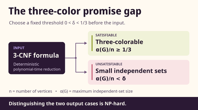
Theorem 1.1 in the original OpenAI preprint fixes any real threshold before the input is chosen. A deterministic polynomial-time reduction takes an explicitly encoded Boolean 3-CNF formula and outputs a nonempty finite simple unweighted graph. It preserves perfect completeness, meaning every satisfiable formula produces an entirely three-colorable graph. Soundness means every unsatisfiable formula produces a graph whose maximum independent set falls strictly below the target density.
The two classes are disjoint because the three-colorable side has an independent set of size at least . A reduction for a fixed rational threshold smaller than the desired real threshold also works for that real threshold. The time and output-size polynomials can have constants and degrees that depend on the threshold. The reduction handles worst-case formulas. The random 3-SAT threshold concerns when random formulas become unsatisfiable.
5. From 3-SAT to Label Cover: Constructing the Hard Instance
The Label Cover reduction replaces the formula with a bipartite system of questions. A label is an answer assigned to one question. Each test occurrence provides a left question, a right question, and a projection that sends every possible left answer to a single right answer. The test passes precisely when that projected answer agrees with the label on the right. The value is the greatest fraction of test occurrences any labeling passes.
The PCP theorem supplies the initial verification gap and parallel repetition drives the unsatisfiable-case value down to any fixed rational tolerance . Satisfiable inputs still admit labels passing every test. The alphabets are constant once the tolerance is fixed. PCP for PPAD uses local verification for a different search problem. Here ordinary total projections suffice, with no bound needed on the number of left answers that share a right image.
6. Layered Tuples and Phase Geometry: Building the Graph
A chain starts with the left questions of a sequence of tests. Each step replaces one question with its right counterpart, and the answer map applies that test’s projection in the replaced position. Other positions stay fixed. At a tuple, a point records a phase for every possible product answer, meaning every combination of labels for its questions. Phases lie on a finite grid of the unit circle, represented modulo one.
Within a tuple’s grid, links have length equal to the largest circle distance across coordinates. Between grids, a target phase vector pulls back by evaluating it at the projected answer for each source coordinate. This pair of points gets a zero-length link. Shortest paths give a pseudometric, since distinct points may have distance zero. An output location sums grid rotations from selected layers, weighted by coefficients and pulled back to the earliest selected layer. Vertices are copies of these locations. Two distinct vertices are adjacent if the distance from one location to the other’s coordinatewise half-shift is at most . An early check returns a clique if any point is that close to its own half-shift. That clique has independence density below the target.
7. Why the Construction Preserves a Proper Three-Coloring
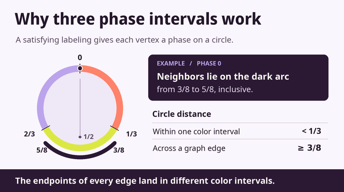
Fix a labeling that passes every test. Each tuple now has a designated product answer. Evaluate a point’s phase at that answer to get a single circle value, written at point . Across a zero-length link, the evaluations agree because the source’s designated answer projects to the target’s. Within a grid, evaluation at one coordinate cannot stretch the maximum coordinate distance. These two facts make evaluation nonexpanding along every path. A point and its half-shift evaluate to opposite phases, so their distance is at least one-half and the clique check cannot trigger.
For an edge with locations and , the evaluated phase of lies within one-eighth of the antipode of the evaluated phase of . The antipode is half a turn away, so the triangle inequality gives the bound below, with denoting circle distance.
Split the circle into three half-open intervals of length and assign one color to each interval. Points in the same interval are closer than one-third, so the endpoints of every edge receive different colors. Every copy at a location receives its location’s color.
8. From Independent Sets to Lipschitz Functions and Juntas
In the soundness case, suppose is a nonempty independent set and the clique check has passed. Its locations stay more than one-eighth away from their half-shifted copies. Build a bump equal to one on those locations and falling linearly with distance until it reaches zero. Subtract its half-shifted version. The resulting grid function is one on the selected locations and flips sign under a half-shift. It has a Lipschitz bound of 64, so changing phases by a small distance changes its value by at most 64 times that distance.
The proof extends each grid function to continuous phases, clips its values to stay between minus one and one, and restores the sign flip. At projected inputs the extensions agree up to a small rounding error, because their grid values already coincide across zero links. Austin’s continuous junta theorem approximates a bounded Lipschitz function on a product cube by a function of a bounded number of coordinates. The bound depends on the Lipschitz constant and error tolerance. That dimension independence is what lets the proof control answer coordinates before fixing the alphabet sizes.
9. Bounded Subchain Lists and the Label Cover Decoding Argument
A junta under independent phase inputs may cease to approximate well after a projection identifies coordinates. The proof therefore works with whole small subchains. Each layer gets its own independent rotation variables, and the subchain function evaluates the weighted sum of pulled-back rotations. The authors approximate this function for each coefficient choice, then take the union of the selected coordinates. The resulting list has at most entries across the subchain and depends only on its own data. Projection to the last layer puts all lists into a common answer space.
Take two subchains with every layer of the first before every layer of the second. Freeze every test except one separating them. The first list depends on that test’s left question, the second on its right question. An intersection after projection means some candidate on the left projects to a candidate on the right. Each pair of list positions defines a labeling strategy once the other tests are fixed, so it succeeds with probability at most . A union bound over at most pairs bounds the intersection probability by .
10. Distributional Alignment: The Key Combinatorial Argument
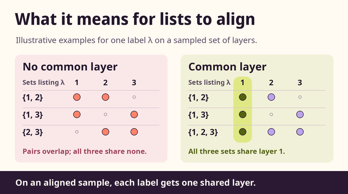
A label can occur on the lists for the pairs {1, 2}, {1, 3}, and {2, 3} without violating disjointness on separated subchains. Yet no layer belongs to all three pairs. The proof needs each label to have a common layer across all the lists containing it within a sampled set. It also needs to fix the sampling law before seeing the lists, since those depend on the independent set under analysis.
The alignment proof records only equality among bounded list slots. Finite minimax says that if no sampling law works, a random allowed pattern can make every set of the chosen size fail with positive probability. Ramsey homogenization and a limiting argument turn these patterns into a random array on rational indices whose law depends only on order. For each label, take the supremum of the minima of its occurrence sets. Separated disjointness bounds that cut between the endpoints of every occurrence set. Order invariance under maps fixing an occurrence set forces the cut onto one of its indices. The common cut contradicts failure. A rational approximation gives the desired finite sampling law.
11. The Geometric Coefficient Test That Forces a Small Independent Set
The analytic test assigns an auxiliary uniform phase to each selected layer, using the common index to decide which phase shifts each answer coordinate. Shifting every auxiliary phase by half a turn negates the function, giving mean zero. Fix an error tolerance with . By Austin’s theorem, mean square above forces some coordinate to have substantial influence, the norm of the difference from averaging out that coordinate. Only a bounded number can meet even half that influence threshold.
Coefficients sit at evenly spaced levels from zero to one with geometrically decreasing probabilities. A layer at coefficient one can absorb the auxiliary shifts by translating its uniform rotations. A fractional coefficient would interfere with taking the shift modulo one. With a full coefficient present, deleting a zero-coefficient layer leaves a subchain whose aligned junta uses no auxiliary phase from the deleted layer. Approximation bounds that layer’s influence. At positive levels, decreasing the coefficient by one step changes influence by less than half the threshold. Each level has probability times the previous one, with . Since few coordinates have that lower influence threshold, large influences at positive levels are rare.
Mean square can exceed only if there is no full coefficient or an influential coordinate appears at zero or at a positive level. Each event has probability below . The squared value is at most one, so the overall mean square is below . The full-coefficient translation removes the auxiliary phases. Samples lacking a full coefficient cost up to one more tolerance, and grid rounding costs another. Since the grid function is one at selected locations, the conditional density on aligned samples is at most .
12. From the Density Bound to NP-Hardness: What the Proof Establishes
Parameters are fixed in dependency order. In particular the list bound comes before the sampling law and the required Label Cover soundness. With source value small enough, the chance of any separated collision is below . The alignment lemma costs at most more, giving unaligned samples probability at most . On unaligned samples the conditional probability of membership is at most one. Integer multiplicities realize the rational sampling law exactly on the vertex set .
Every proper coloring partitions the graph into independent classes of size at most . Their sizes sum to , yielding the chromatic number bound.
Choose for a fixed palette size . The soundness bound forces , ruling out that palette, while satisfiable inputs already have a three-coloring. OpenAI published it with its October mathematics release. The Lean scope note for family 106 describes formalization of the reduction, including the cost of the full adjacency-matrix output. Its proof gives no practical runtime benchmark, and growing palettes remain compatible with it.
Graph coloring is NP-hard under this promise because phase geometry preserves a three-coloring in the satisfiable case while the alignment and coefficient arguments rule out even one large color class in the unsatisfiable case. Follow Binary Verse AI for more research explainers on graph refinement lower bounds and approximation hardness in bin packing.
Is graph coloring NP-hard even when a graph is known to be three-colorable?
Yes. The proof establishes NP-hardness of finding a proper coloring with any fixed palette of three or more colors, even when the input is promised to be three-colorable.
Why does every three-colorable graph contain a large independent set?
A proper three-coloring partitions the vertices into three color classes. At least one contains at least one-third of the vertices. No two vertices in that class share an edge, so it is an independent set.
What is the chromatic number, and how is it related to independent sets?
The chromatic number is the smallest palette size of a proper coloring. Each color class is independent, so the chromatic number is at least the total number of vertices divided by the maximum independent-set size.
Why doesn’t allowing more colors eliminate the computational difficulty?
For every fixed palette size, the reduction can make the largest independent set in the hard case smaller than the average class size that palette would require. The result applies to fixed palettes. A palette that grows with graph size falls outside that guarantee.
What makes the OpenAI proof different from earlier graph-coloring results?
Earlier work established fixed-palette hardness. This paper also makes the maximum independent-set density arbitrarily small in the unsatisfiable case while retaining a proper three-coloring of every vertex in the satisfiable case.
How can the proof use random phases and coefficients yet produce a deterministic reduction?
The graph construction enumerates a finite experiment with rational probabilities. A common denominator turns those probabilities into integer vertex multiplicities. The continuous phases used in the soundness proof enter the analysis only.
Does this proof mean that efficient graph-coloring algorithms are impossible?
It rules out a polynomial-time algorithm with the stated fixed-palette worst-case guarantee unless P equals NP. Heuristics, algorithms for restricted graph classes, and algorithms using palettes that grow with graph size remain possible.